1 Dataset explanation
This dataset was created using a fresh frozen eyeball issue sample from a mouse (Strain: C57BL/6; Sex: Male; Age: 6-8 week), using a Kit version Stereo-seq T FF V1.3 on a ship size : 0.5 cm × 0.5 cm with a section thickness of 10 μm and H&E staining. You can find more information here
2 Download dataset
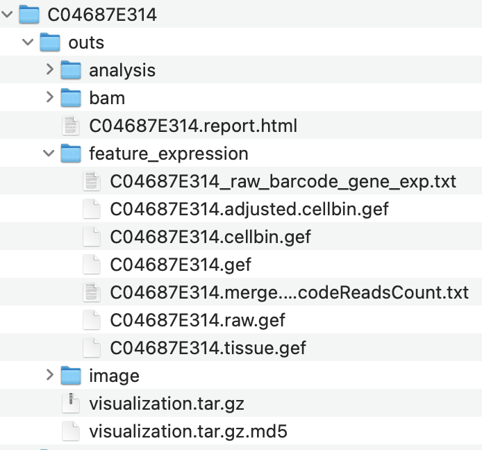
Download the dataset from the STOmics website. The demo data has a different file structure than data coming from a real sequencing experiment. Once you have downloaded the demo dataset, please re-arrange the files to use the Giotto reader, your folder should look similar to this:
3 Set up Giotto environment
Ensure that the Giotto package is installed. Additionally, check that the mini conda Giotto environment with Python dependencies is installed.
If you have installation troubles, visit the Installation and Frequently Asked Questions sections.
# Ensure Giotto Suite is installed.
if(!"Giotto" %in% installed.packages()) {
  pak::pkg_install("giotto-suite/Giotto")
}

# Ensure the Python environment for Giotto has been installed.
genv_exists <- Giotto::checkGiottoEnvironment()
if(!genv_exists){
  # The following command need only be run once to install the Giotto environment.
  Giotto::installGiottoEnvironment()
}

library(Giotto)
4 Set the Giotto instructions
{Giotto} instructions are used to apply settings to giotto object behavior at the project level. Each giotto object needs a set of instructions information that can either be manually set or generated with defaults when the giotto object is first created. Once added, these instructions are stored in the giotto object @instructions slot.
# Set the results directory to save plots
results_folder <- "path/to/results"

# Optional: Specify the path to a Python executable within a conda or miniconda
# environment. If set to NULL (default), the Python executable within the previously installed Giotto environment will be used.
python_path <- NULL # alternatively, "/local/python/path/python" if desired.

# Create Giotto Instructions
instructions <- createGiottoInstructions(save_dir = results_folder,
                                         save_plot = TRUE,
                                         show_plot = FALSE,
                                         return_plot = FALSE,
                                         python_path = python_path)
The stereo-seq readers will look for the standardized files organization from the STOmics technology in the data folder and will automatically load the expression and spatial information to create the Giotto object.
## provide a path to your sample data. It should point to the "outs" subfolder under your main data folder.
data_path <- "/path/to/outs/"
5 Create the Giotto object using the reader
This step will read multiple components at the same time and will create a Giotto object. You can create multiple combinations of the data, e.g. the expression matrix and spatial locations only (by setting load_image = FALSE and load_mask = FALSE).
reader_bin <- importStereoSeq(stereoseq_dir = data_path)

g <- reader_bin$create_gobject(
  load_expression = TRUE,
  load_spatlocs = TRUE,
  load_image = TRUE,
  load_mask = TRUE,
  verbose = TRUE,
  instructions = instructions)
Visualize the object.
spatPlot2D(g,
           show_image = TRUE,
           point_size = 4)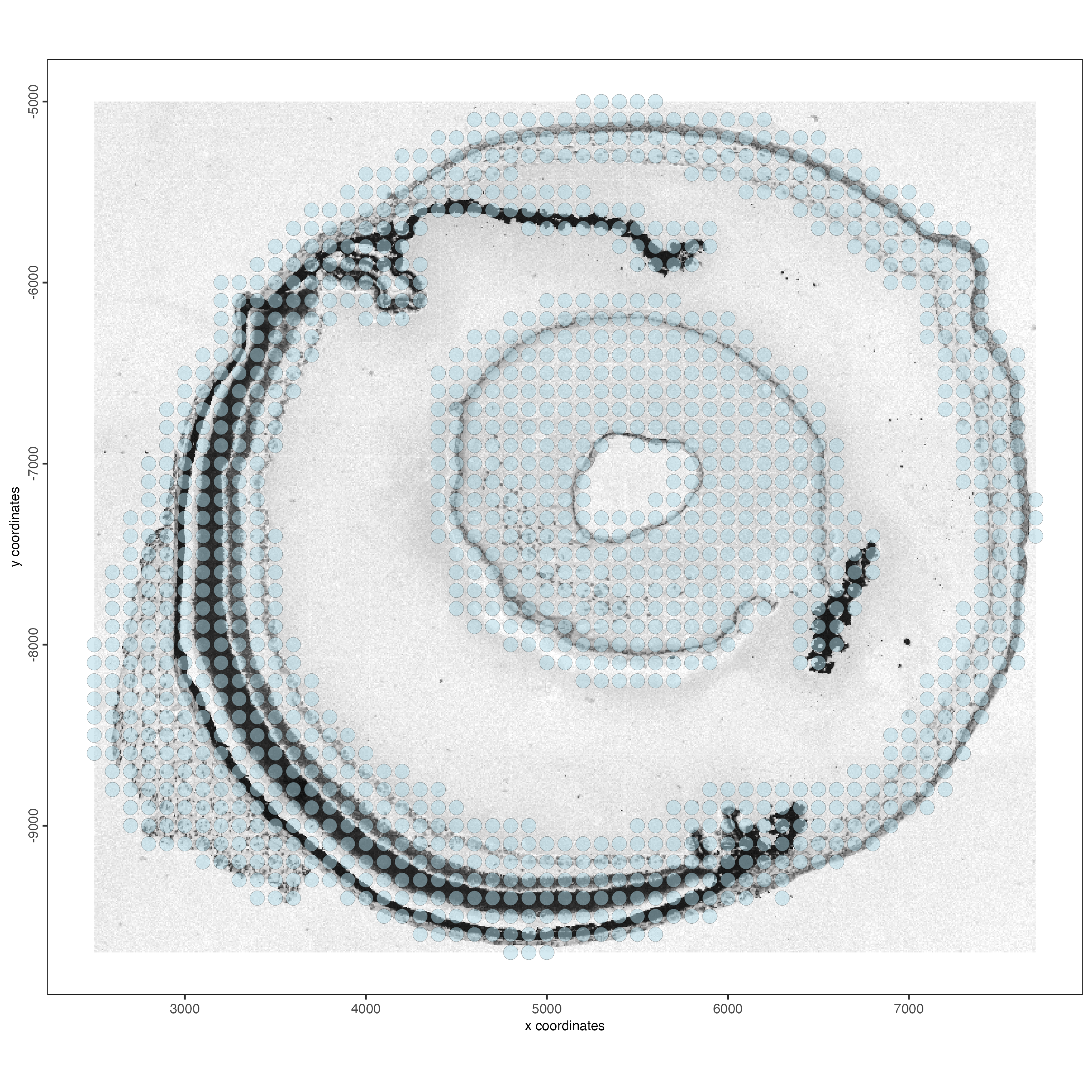
6 Read bin data using individual loaders
When reading the expression information at the bin level, you can select from different resolutions (e.g. “bin1”, “bin5”, “bin10”, “bin20”, “bin50”, “bin100”, “bin150”, or “bin200”).
6.1 Start the reader for bin-level data
Some recommendations for using the reader:
- Make sure to set: type = “bin”.
- The default bin size is “bin100”, list the available bins in your sample with ’rhdf5::h5ls(“/path/to/*.tissue.gef”)’.
- gene_column will determine if your features/genes use the common gene name (gene_column = “geneName”) or an ENSEMBL id (gene_column = “geneID”).
- negative_y will control if the spatial y-coordinates are represented
in the negative (negative_y = TRUE) or positive (negative_y = FALSE)
space. You can see the difference when plotting your sample with
spatPlot2D().
reader_bin <- importStereoSeq(
  stereoseq_dir = data_path,
  type = "bin",
  bin_size = "bin100",
  gene_column = "geneName",
  negative_y = TRUE
)
6.2 Load expression
The output of this step will be an exprObj with the raw expression matrix (feature/gene x bin). At this bin size, this dataset has 1309 bins and 26535 genes.
expr_bin <- reader_bin$load_expression(verbose = TRUE)6.3 Load spatial locations
The output of this step will be an spatLocsObj with the spatial coordinates of each bin.
spatlocs_bin <- reader_bin$load_spatlocs(verbose = TRUE)6.4 Load image
The output of this step will be a giottoLargeImage with the HE image.
img_bin <- reader_bin$load_image(verbose = TRUE)6.5 Load mask
The output of this step will be a giottoPolygon with the cell boundaries from the *HE_mask.tiff file.
mask_poly <- reader_bin$load_mask(verbose = TRUE)6.6 Assemble the object
Use the individual pieces to create a custom Giotto object.
g_bin <- giotto()
g_bin <- setGiotto(g_bin, expr_bin, verbose = TRUE)
g_bin <- setGiotto(g_bin, spatlocs_bin, verbose = TRUE)
g_bin <- setGiotto(g_bin, mask_poly, verbose = TRUE)
g_bin <- setGiotto(g_bin, img_bin, verbose = TRUE)
This object has the default instructions. You can set the instructions we defined at the beginning of the tutorial using the instructions() function.
instructions(g_bin) <- instructionsVisualize the object
spatPlot2D(g_bin,
           show_image = TRUE,
           point_size = 4)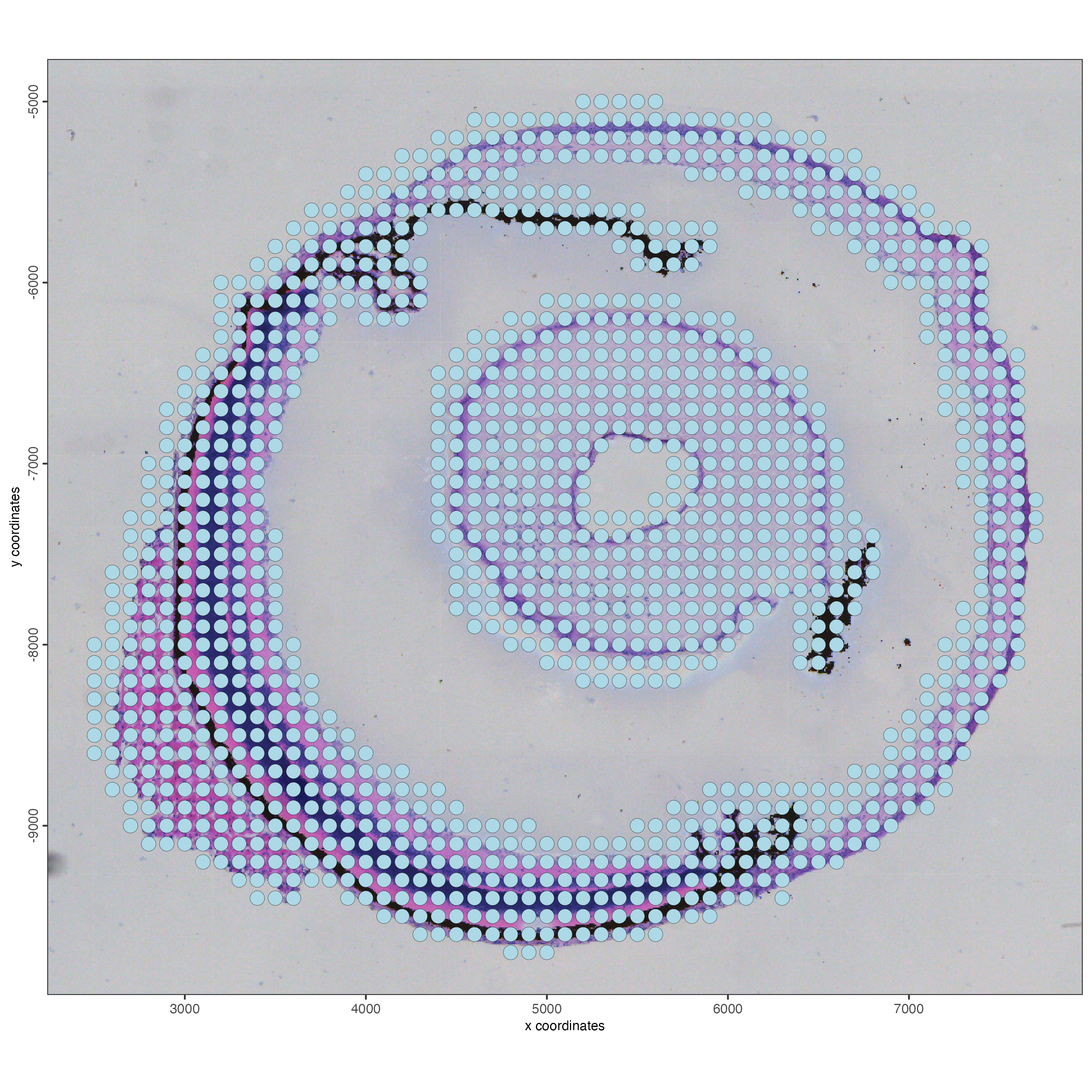
7 Read bin data using the convenience function
Read the bin expression matrix, spatial locations, image, and polygons in one step.
Use gef_type = “tissue” (default) to read only the bins that overlap with the tissue area.
g_bin <- createGiottoStereoSeqObjectBin(
    stereoseq_dir = data_path,
    bin_size = "bin100",
    gef_type = "tissue",
    load_image = TRUE,
    load_mask = TRUE,
    verbose = TRUE,
    instructions = instructions
  )
Visualize the bins.
spatPlot2D(g_bin,
           show_image = TRUE,
           point_size = 4)
Use gef_type = “full” to read all the bins, including those out of the tissue area.
g_bin <- createGiottoStereoSeqObjectBin(
    stereoseq_dir = data_path,
    bin_size = "bin100",
    gef_type = "full",
    load_image = TRUE,
    load_mask = TRUE,
    verbose = TRUE,
    instructions = instructions
  )
Visualize the bins.
spatPlot2D(g_bin,
           show_image = TRUE,
           point_size = 1)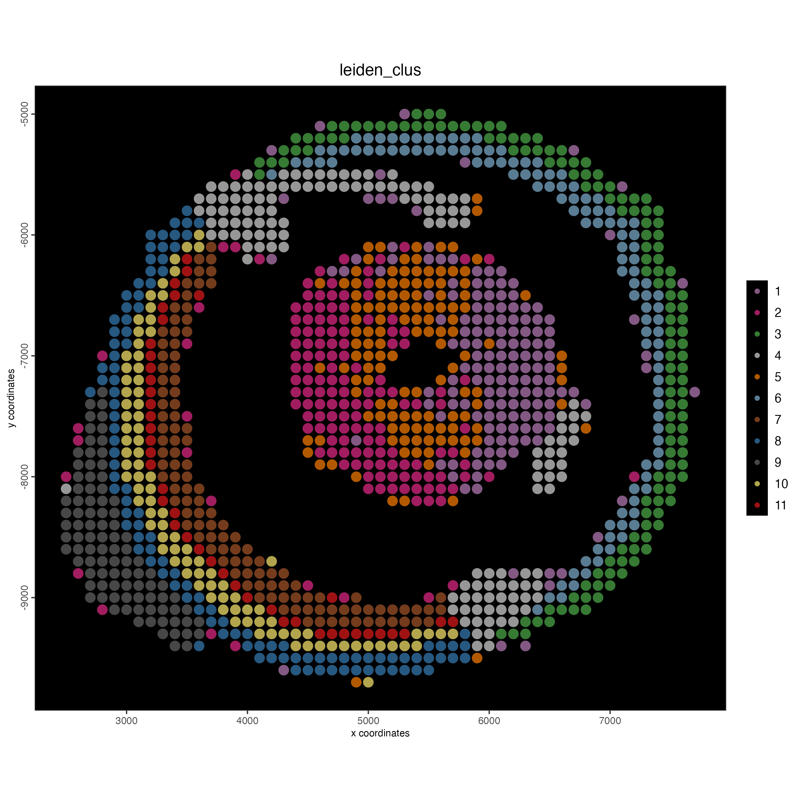
8 Read cell data using individual loaders
8.1 Start the reader for cell-level data
Some recommendations for using the reader:
- Make sure to set: type = “cell”.
- No need to use the “bin” argument in this scenario.
- gene_column will determine if your features/genes use the common gene name (gene_column = “geneName”) or an ENSEMBL id (gene_column = “geneID”).
- negative_y will control if the spatial y-coordinates are represented
in the negative (negative_y = TRUE) or positive (negative_y = FALSE)
space. You can see the difference when plotting your sample with
spatPlot2D().
reader_cell <- importStereoSeq(
  stereoseq_dir = data_path,
  type = "cell",
  gene_column = "geneName",
  negative_y = TRUE
)
8.2 Load expression
The output of this step will be an exprObj with the raw expression matrix (feature/gene x cell). At the cell size, this dataset has 7527 cells and 25646 genes.
expr_cell <- reader_cell$load_expression(verbose = TRUE)8.3 Load spatial locations
The output of this step will be an spatLocsObj with the spatial coordinates of each cell.
spatlocs_cell <- reader_cell$load_spatlocs(verbose = TRUE)8.4 Load image
The output of this step will be a giottoLargeImage with the HE image.
img_cell <- reader_cell$load_image(verbose = TRUE)8.5 Load cell border polygons
The output of this step is a giottoPolygon object with the cell polygons, result of the cell segmentation.
poly <- reader_cell$load_polygons(verbose = TRUE)8.6 Assemble the object
Use the individual pieces to create a custom Giotto object.
g_cell <- giotto()
g_cell <- setGiotto(g_cell, expr_cell, verbose = TRUE)
g_cell <- setGiotto(g_cell, spatlocs_cell, verbose = TRUE)
g_cell <- setGiotto(g_cell, poly, verbose = TRUE)
g_cell <- setGiotto(g_cell, img_cell, verbose = TRUE)
Set the Giotto instructions
instructions(g_cell) <- instructionsVisualize the object
spatPlot2D(g_cell,
           show_image = TRUE,
           point_size = 1)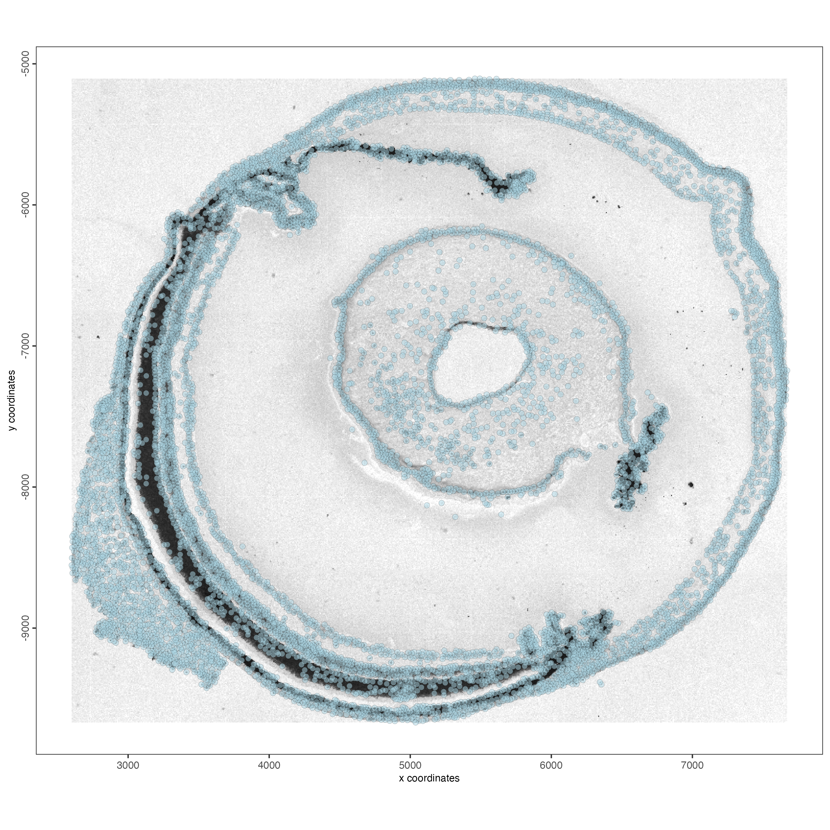
9 Read cell data using the convenience function
g_cell <- createGiottoStereoSeqObjectCell(
    stereoseq_dir = data_path,
    gef_type = "adjusted_cellbin",  # default
    load_polygons = TRUE,
    load_mask = FALSE,
    load_image = TRUE,
    verbose = TRUE,
    negative_y = TRUE,
    instructions = instructions
  )
Visualize the object
spatPlot2D(g_cell,
           show_image = TRUE,
           point_size = 1)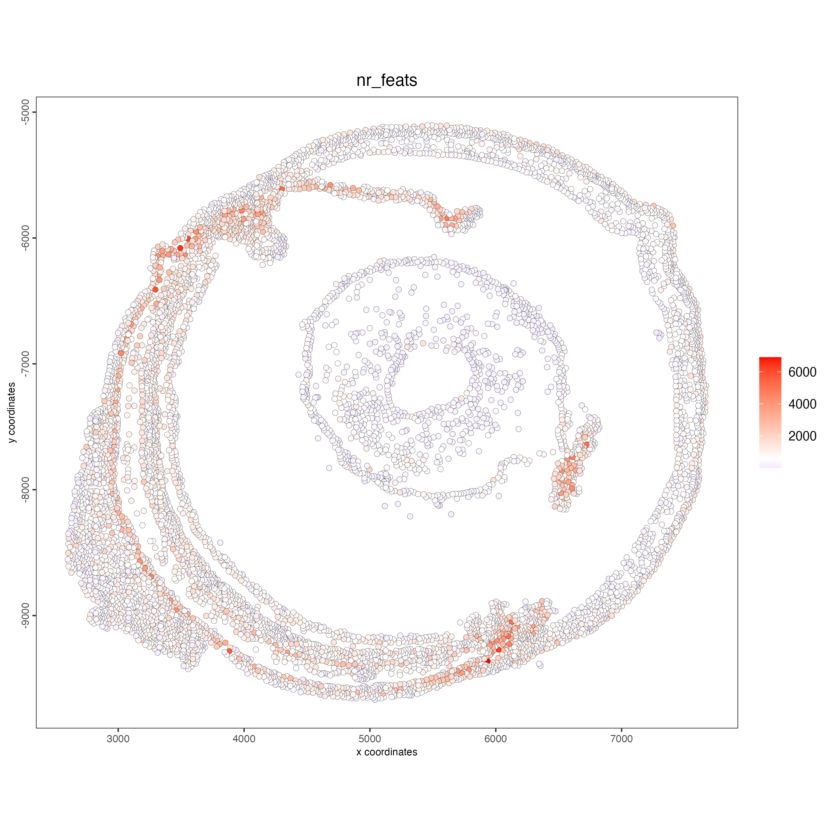
10 Read subcellular data using individual loaders
10.1 Load subcellular bin data as binpoints
Read the smallest bin size (bin1) and create a giottoBinPoints object.
gbp_bin <- reader_bin$load_binpoints(verbose = TRUE)10.2 Load mask polygons
The output of this step is a giottoPolygon object.
mask_poly <- reader_bin$load_mask(verbose = TRUE)10.3 Load image
The output of this step will be a giottoLargeImage with the HE image.
img_bin <- reader_bin$load_image(verbose = TRUE)10.4 Assemble the object
The resulting object will only contain subcellular data. The aggregated matrix can be calculated using downstream steps.
g_sub <- giotto()
g_sub <- setGiotto(g_sub, gbp_bin, verbose = TRUE)
g_sub <- setGiotto(g_sub, mask_poly, verbose = TRUE)
g_sub <- setGiotto(g_sub, img_cell, verbose = TRUE)
Print the object and note there’s only feature data in the subcellular info, but the aggregated info only contains the image.
g_subOverlap the subcellular info with the cell segmentation polygons to create an aggregated expression matrix.
Find the feature points overlapped by polygons. This overlap information is then returned to the relevant giottoPolygon object’s overlaps slot.
g_sub <- calculateOverlap(
  g_sub,
  spat_info = "cell",
  feat_info = "rna"
)
Convert the overlap information into a cell by feature expression matrix which is then stored in the Giotto object’s expression slot.
g_sub <- overlapToMatrix(
  g_sub,
  spat_info = "cell",
  feat_info = "rna",
  name = "raw"
)
Print the object again and note the aggregated info with raw counts.
g_subSet the Giotto instructions and visualize the aggregated object at the cell level.
instructions(g_sub) <- instructions

spatPlot2D(g_sub,
           show_image = TRUE,
           point_size = 1)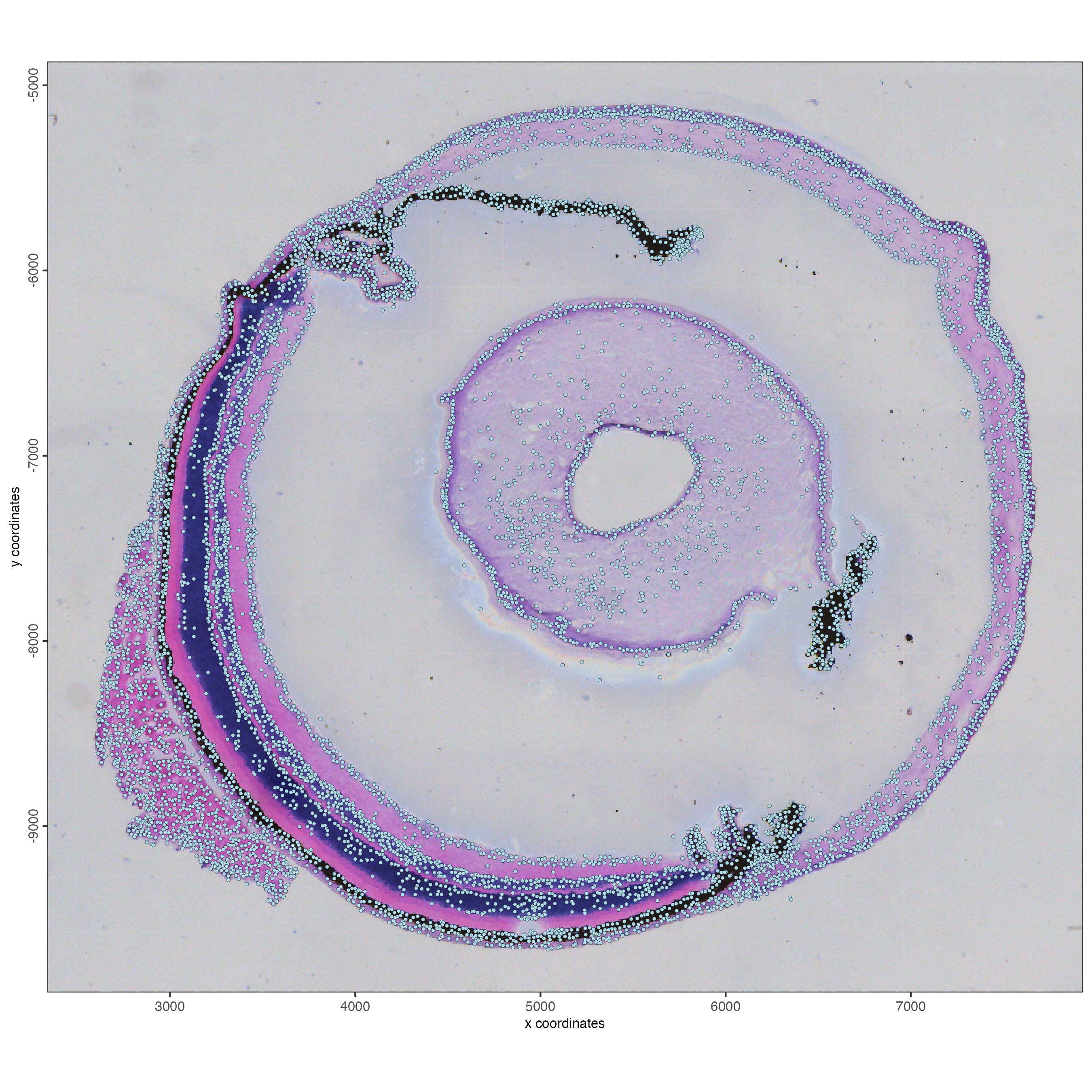
11 Create a Giotto object using subcellular and cell segmentation data
Read both the mask and giottoBinPoints in a single step, then run a second step to aggregate the data at the cell-level expression matrix.
g_sub <- reader_bin$create_gobject(
  load_expression = FALSE,
  load_spatlocs = FALSE,
  load_image = TRUE,
  load_mask = TRUE,
  load_binpoints = TRUE,
  verbose = TRUE,
  instructions = instructions)
Print the object and note there’s only subcellular info.
g_subCalculate the overlap with cell polygons and the aggregated matrix.
g_sub <- calculateOverlap(
  g_sub,
  spat_info = "cell",
  feat_info = "rna"
)
g_sub <- overlapToMatrix(
  g_sub,
  spat_info = "cell",
  feat_info = "rna",
  name = "raw"
)
Print the object again and note the aggregated info with raw counts.
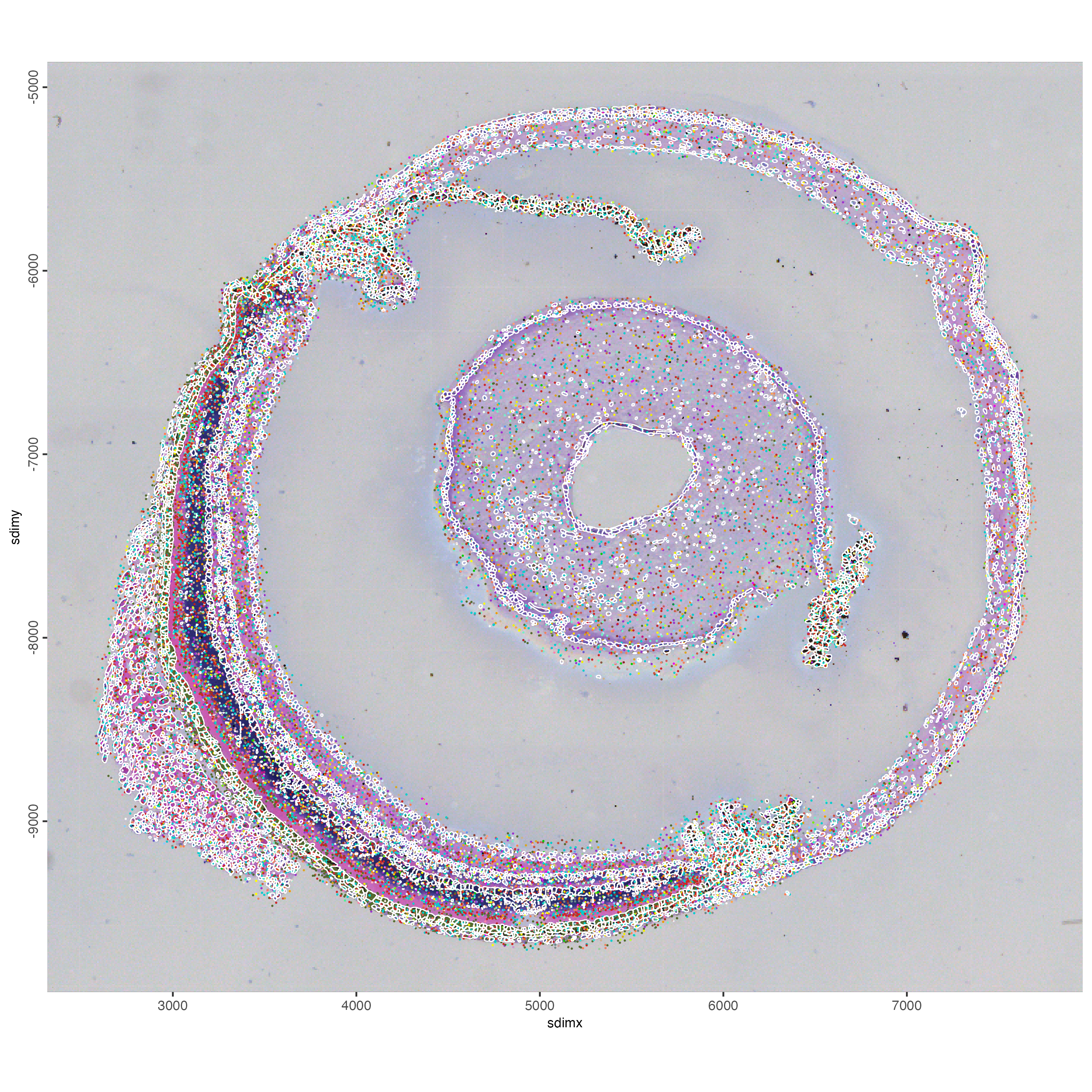
g_subVisualize the cell polygons and some genes. You can select genes to plot their location across the sample. spatInSituPlotPoints will also plot the segmentation cell boundaries stored as Giotto Polygons.
genes <- featIDs(g_sub)
selected_genes <- genes[sample(size = 100, x = 1:length(genes))]

spatInSituPlotPoints(
  gobject = g_sub,
  show_image = TRUE,
  image_name = "image",
  show_polygon = TRUE,
  polygon_feat_type = "cell",
  polygon_color = "white",
  polygon_alpha = 0,
  polygon_line_size = 0.3,
  feats = list('rna' = selected_genes),
  use_overlap = FALSE,
  show_legend = FALSE,
  spat_unit = "cell",
  point_size = 0.3
)
12 Read subcellular data using the convenience function
When using createGiottoStereoSeqObjectBin(), load_binpoints = TRUE will read the smallest resolution bin (bin1) as giottoBinPoints, while load_mask = TRUE will load the cell polygons. This information will be used in a downstream step to aggregate the bin1 counts at the cellular level.
Optionally, you can also read the expression matrix at any bin resolution. In this example, we are also loading the bin1 expression by setting bin_size = “bin1” and load_expression = TRUE.
g_sub <- createGiottoStereoSeqObjectBin(
    stereoseq_dir = data_path,
    bin_size = "bin1", # smallest resolution expression matrix
    gef_type = "tissue",
    load_expression = TRUE, # bin1 expression matrix
    load_spatlocs = TRUE,
    load_binpoints = TRUE, # bin1 giottoBinPoints (0.5 µm DNBs)
    load_image = TRUE,
    load_mask = TRUE, # cell polygons from HE mask
    verbose = TRUE,
    instructions = instructions
  )
Print the object and note that the aggregated info only contains the bin1 level, but not cellular level.
g_subOverlap the giottoBinPoints and cell polygons.
g_sub <- calculateOverlap(
    g_sub,
    spat_info = "cell",
    feat_info = "rna"
  )

g_sub <- overlapToMatrix(
    g_sub,
    spat_info = "cell",
    feat_info = "rna",
    name = "raw"
  )
Print the object again and note that the aggregated info now contains both the bin1 and cellular level.
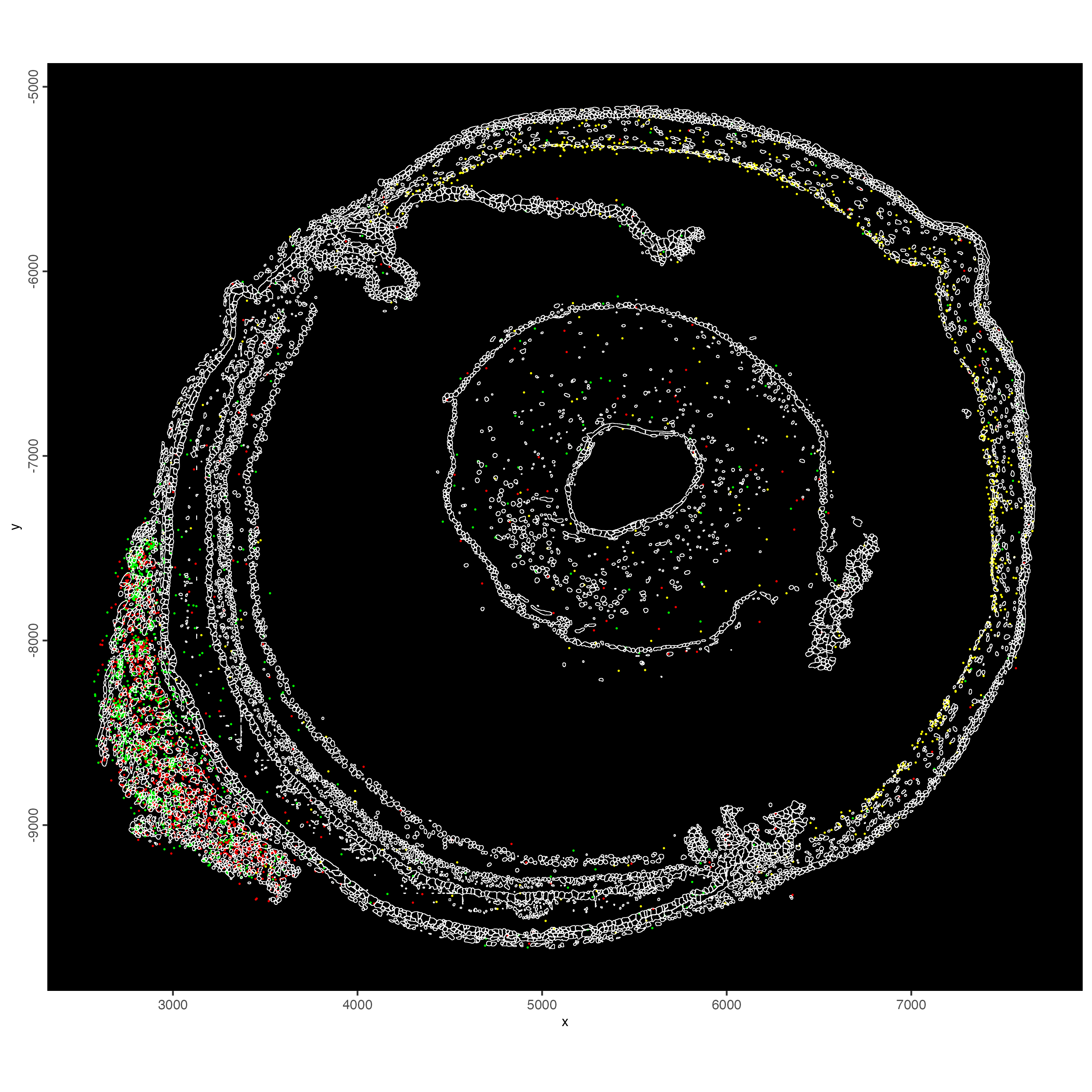
g_subVisualize the cell polygons and some genes.
spatInSituPlotPoints(g_sub,
                     spat_unit = "cell",
                     show_image = FALSE,
                     show_polygon = TRUE,
                     polygon_feat_type = "cell",
                     polygon_color = "white",
                     polygon_alpha = 0,
                     polygon_line_size = 0.2,
                     feats = list("rna" = c("Slc4a11", "Myh7", "Mylk4")),
                     feats_color_code = c("Slc4a11" = "yellow",
                                          "Myh7" = "green",
                                          "Mylk4" = "red"),
                     point_size = 0.3,
                     use_overlap = FALSE,
                     show_legend = FALSE,
                     background_color = "black"
)
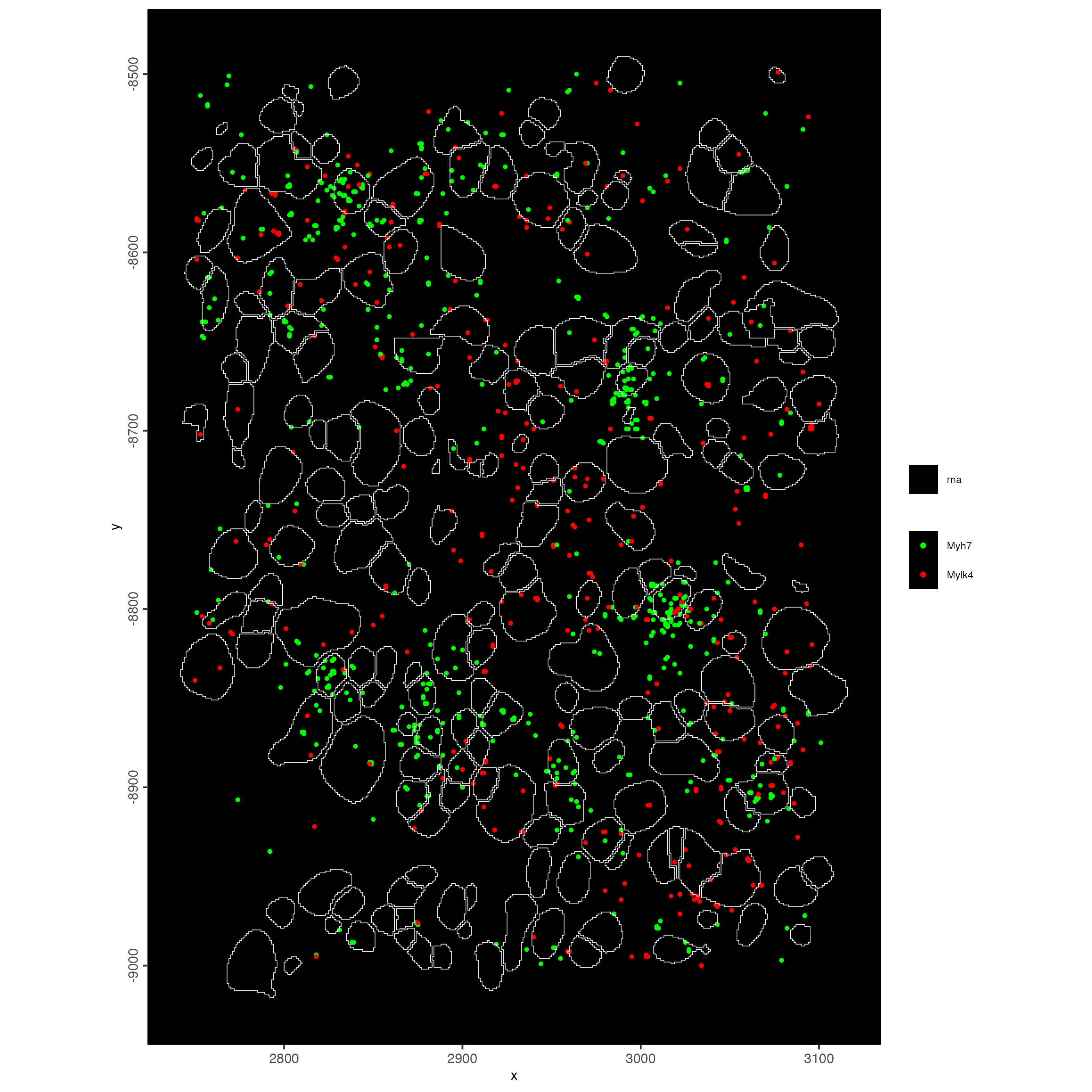
Use subsetGiottoLocsSubcellular to subset a specific region of the sample and obtain a zoomed in visualization of the transcripts.
g_subset <- subsetGiottoLocs(g_sub,
                             spat_unit = "cell",
                             x_min = 2750,
                             x_max = 3100,
                             y_min = -9000,
                             y_max = -8500)

spatInSituPlotPoints(g_subset,
                     spat_unit = "cell",
                     show_image = FALSE,
                     show_polygon = TRUE,
                     polygon_feat_type = "cell",
                     polygon_color = "white",
                     polygon_alpha = 0,
                     polygon_line_size = 0.2,
                     feats = list("rna" = c("Myh7", "Mylk4")),
                     feats_color_code = c("Myh7" = "green",
                                          "Mylk4" = "red"),
                     expand_counts = TRUE,
                     count_info_column = "count",
                     jitter = c(1, 1),
                     point_size = 1,
                     use_overlap = FALSE,
                     background_color = "black"
)
13 Process the Giotto object at the cell level
13.1 Quality control
Use the function addStatistics() to count the number of features per cell. The statistics information will be stored in the metadata table under the new column “nr_feats”. Then, use this column to visualize the number of features per cell across the sample.
g_statistics <- addStatistics(gobject = g_cell,
                              expression_values = "raw")

## visualize
spatPlot2D(gobject = g_statistics,
           point_size = 2,
           cell_color = "nr_feats",
           color_as_factor = FALSE)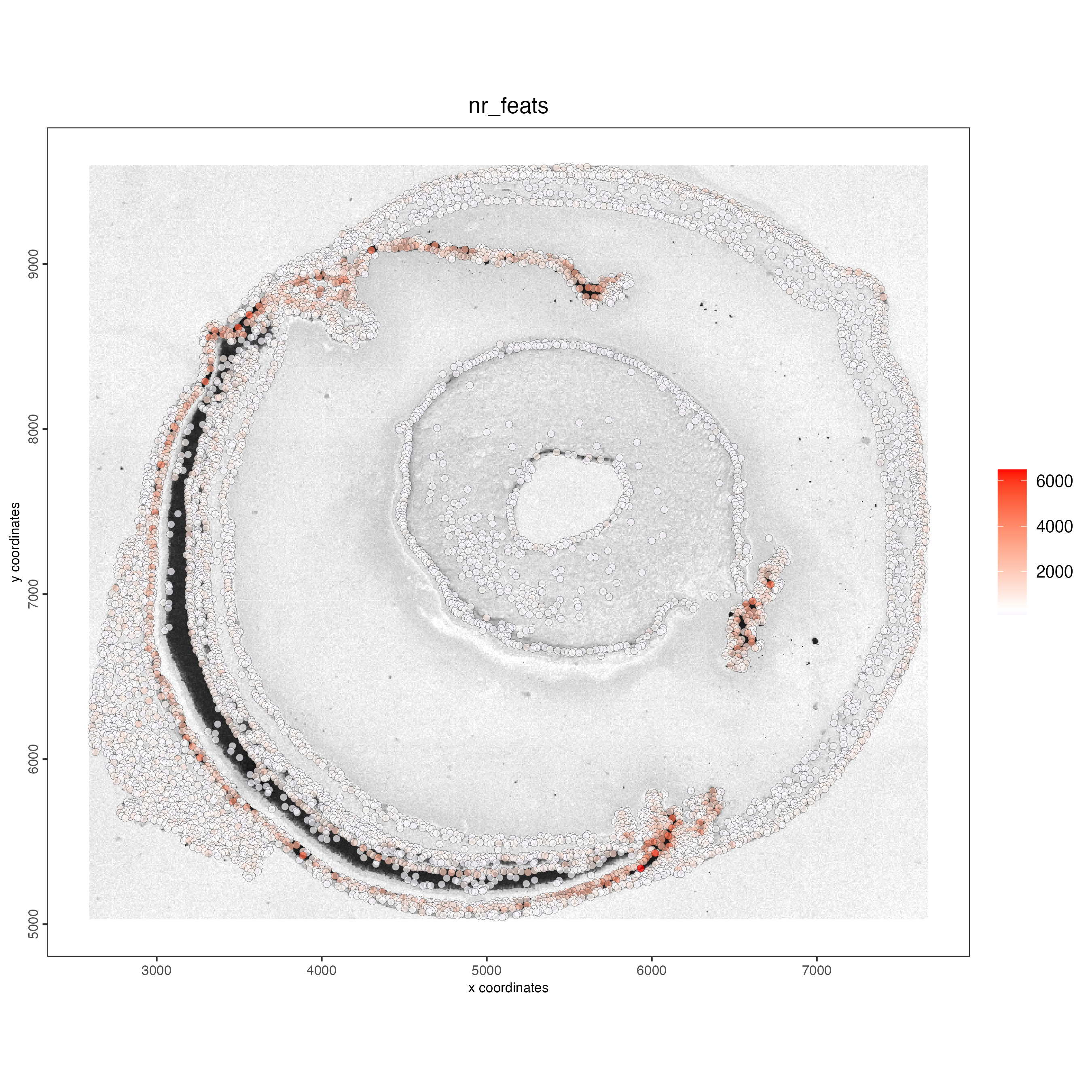
filterDistributions() creates a histogram to show the distribution of features per cell across the sample.
filterDistributions(gobject = g_statistics,
                    detection = "cells")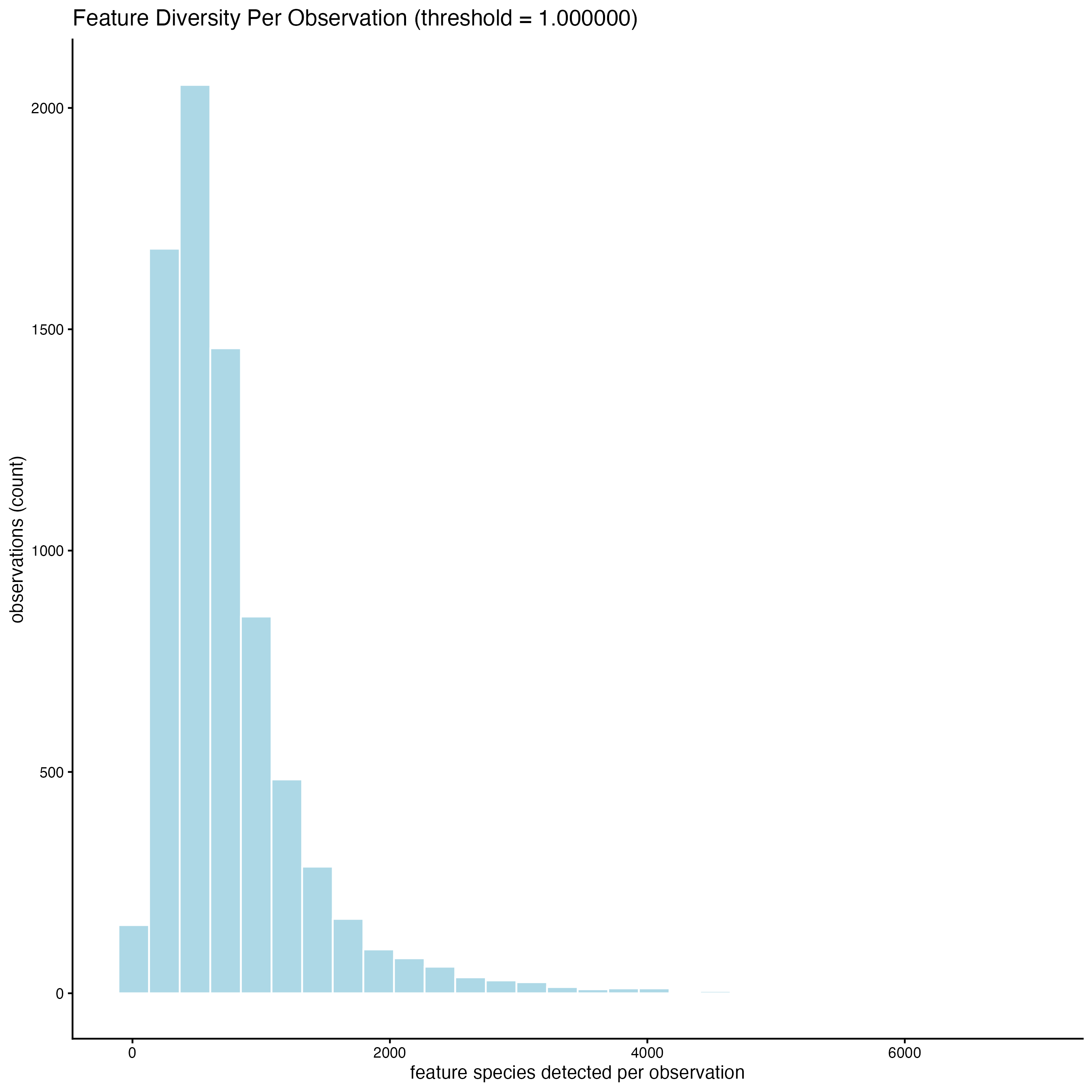
When setting the detection = “feats”, the histogram shows the distribution of cells with certain number of features across the sample.
filterDistributions(gobject = g_statistics,
                    detection = "feats")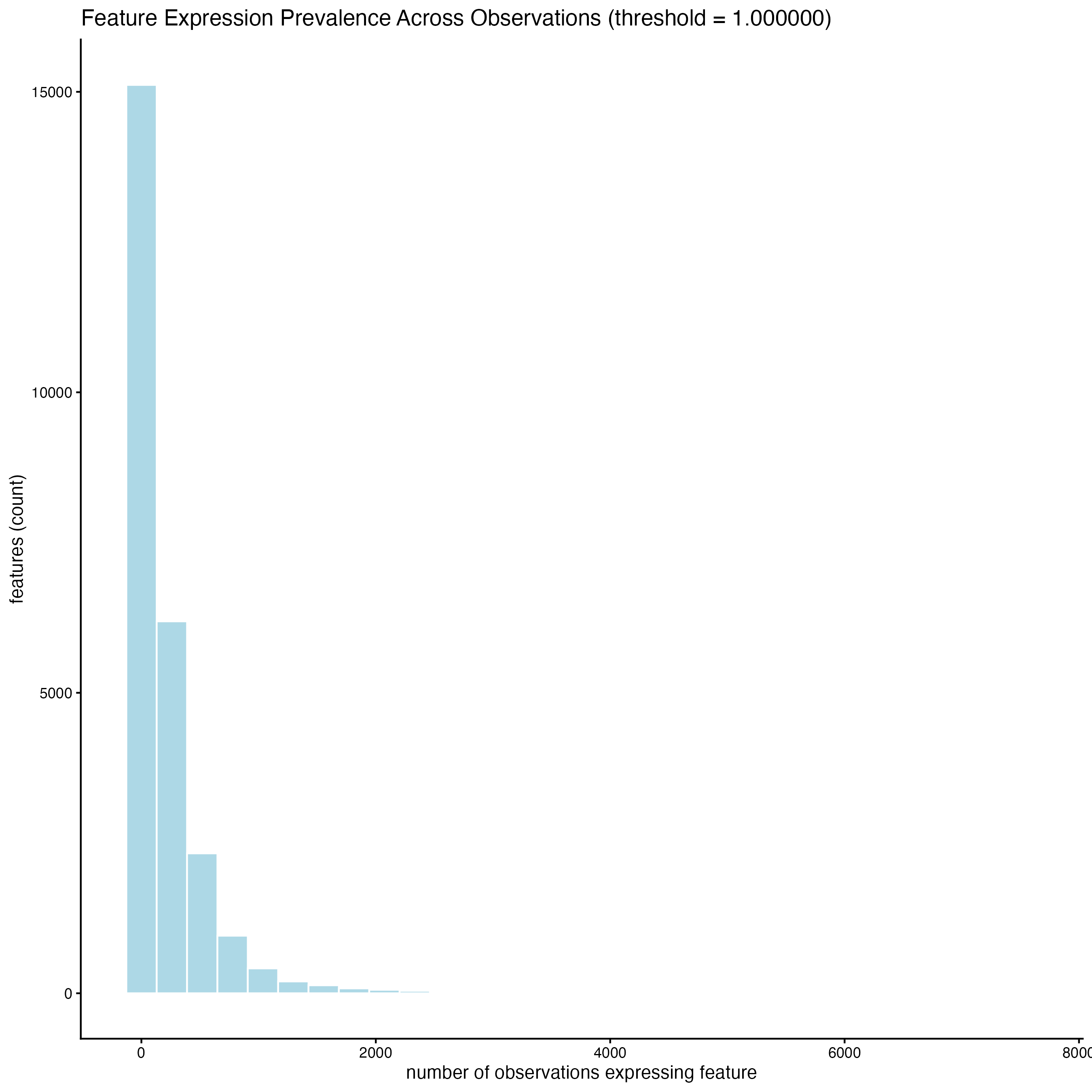
13.2 Filtering
Use the arguments feat_det_in_min_cells and min_det_feats_per_cell to set the minimal number of cells where an individual feature must be detected and the minimal number of features per cell, respectively, to filter the giotto object. All the features and cells under those thresholds will be removed from the sample.
g_cell <- filterGiotto(gobject = g_cell,
                       expression_threshold = 1,
                       feat_det_in_min_cells = 10,
                       min_det_feats_per_cell = 100,
                       expression_values = "raw",
                       verbose = TRUE)
13.3 Normalization
Use scalefactor to set the scale factor to use after library size normalization. The default value is 6000, but you can use a different one.
g_cell <- normalizeGiotto(gobject = g_cell,
                          scalefactor = 6000,
                          verbose = TRUE)
Calculate the normalized number of features per cell and save the statistics in the metadata table.
g_cell <- addStatistics(gobject = g_cell)

## visualize
spatPlot2D(gobject = g_cell,
           point_size = 2,
           show_image = TRUE,
           point_alpha = 0.7,
           cell_color = "nr_feats",
           color_as_factor = FALSE)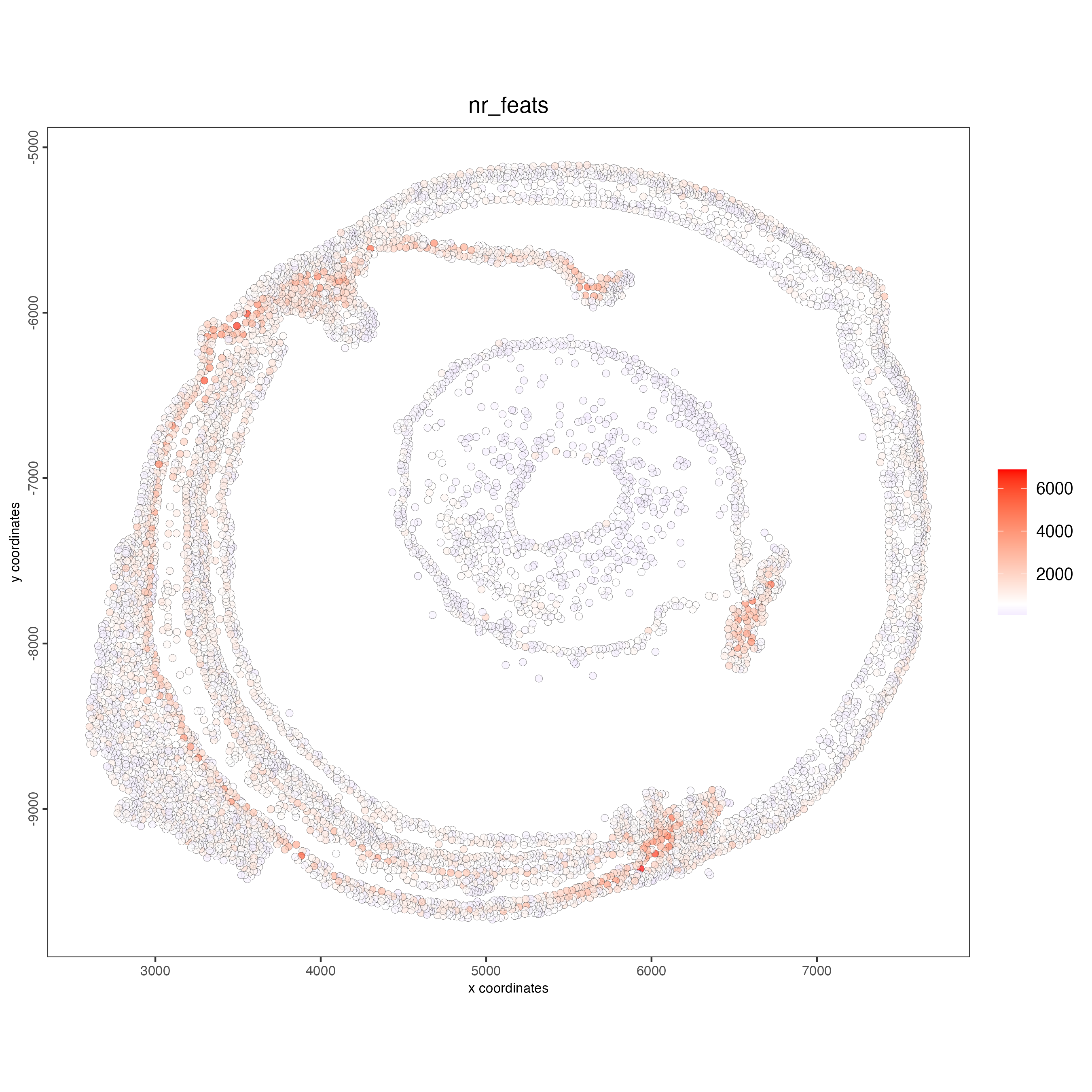
You can also visualize the number of transcripts per cell.
spatPlot2D(gobject = g_cell,
           point_size = 2,
           show_image = TRUE,
           point_alpha = 0.7,
           cell_color = "total_expr",
           color_as_factor = FALSE)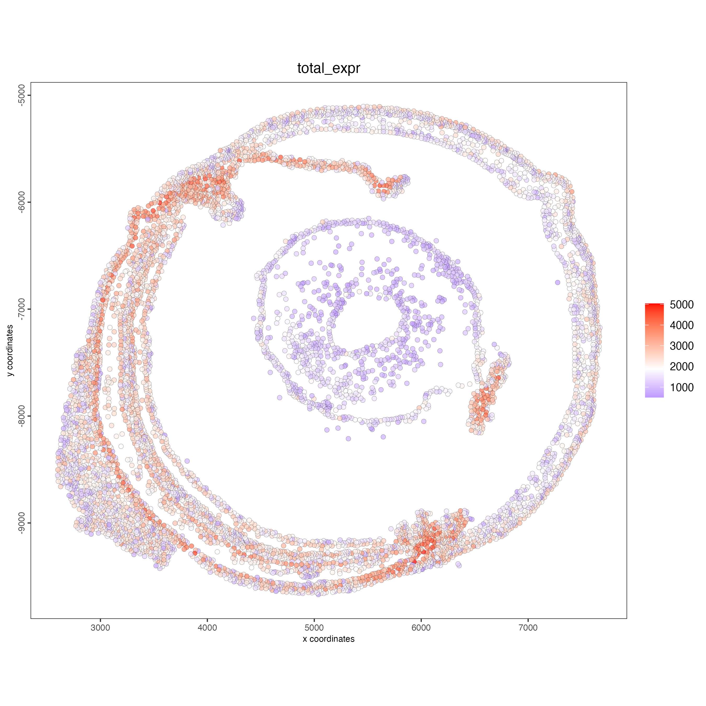
13.4 Feature selection
Calculating Highly Variable Features (HVF) is necessary to identify genes (or features) that display significant variability across the cells.
g_cell <- calculateHVF(gobject = g_cell,
                       save_plot = TRUE)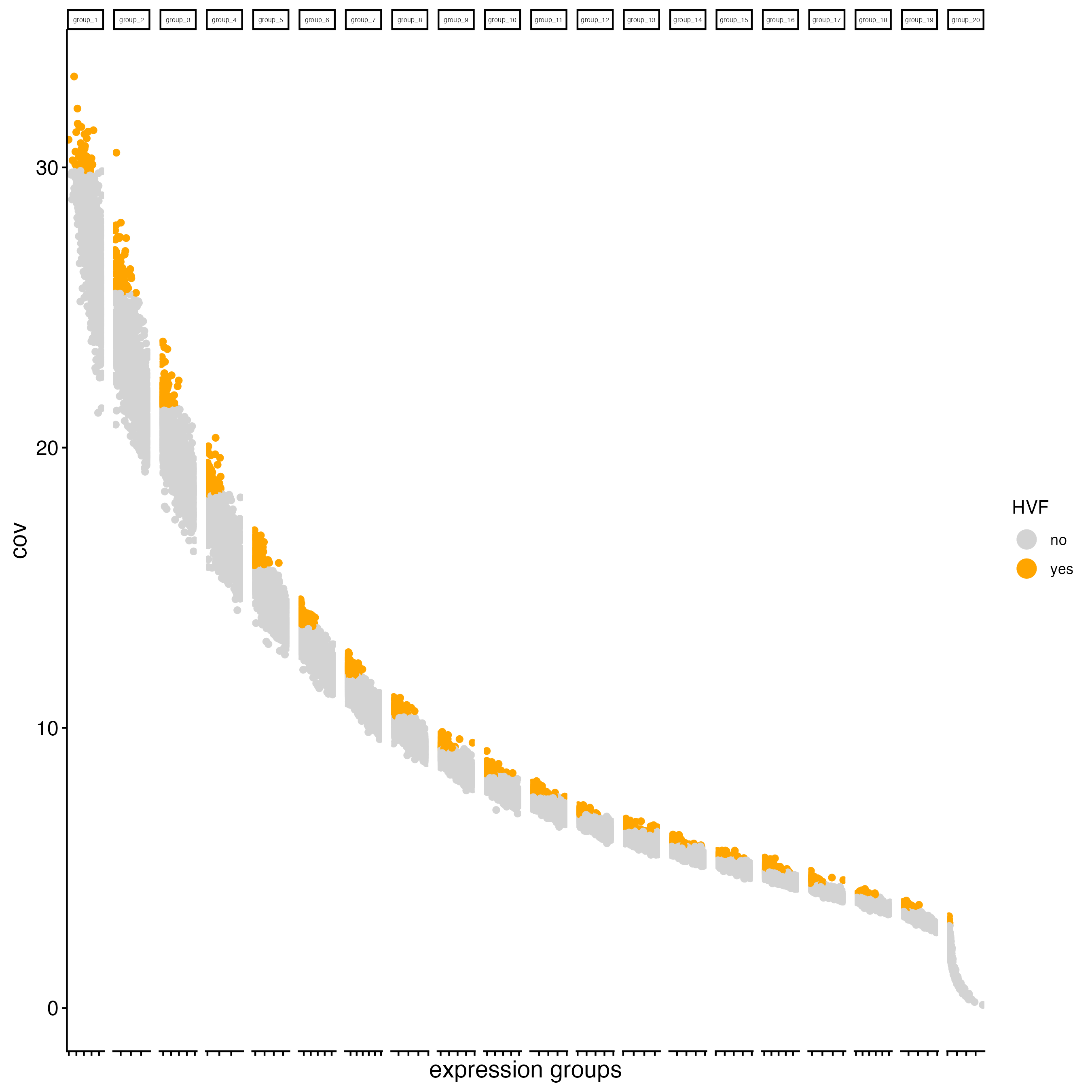
13.5 Dimension reduction
13.5.1 PCA
Principal Components Analysis (PCA) is applied to reduce the dimensionality of gene expression data by transforming it into principal components, which are linear combinations of genes ranked by the variance they explain, with the first components capturing the most variance.
- runPCA() will look for the previous calculation of highly variable features, stored as a column in the feature metadata. If the HVF labels are not found in the giotto object, or the parameter “feats_to_use” is set to NULL, then runPCA() will use all the features available in the sample to calculate the Principal Components.
g_cell <- runPCA(gobject = g_cell,
                 ncp = 50)
Create a screeplot to visualize the percentage of variance explained by each component.
screePlot(gobject = g_cell,
          ncp = 50)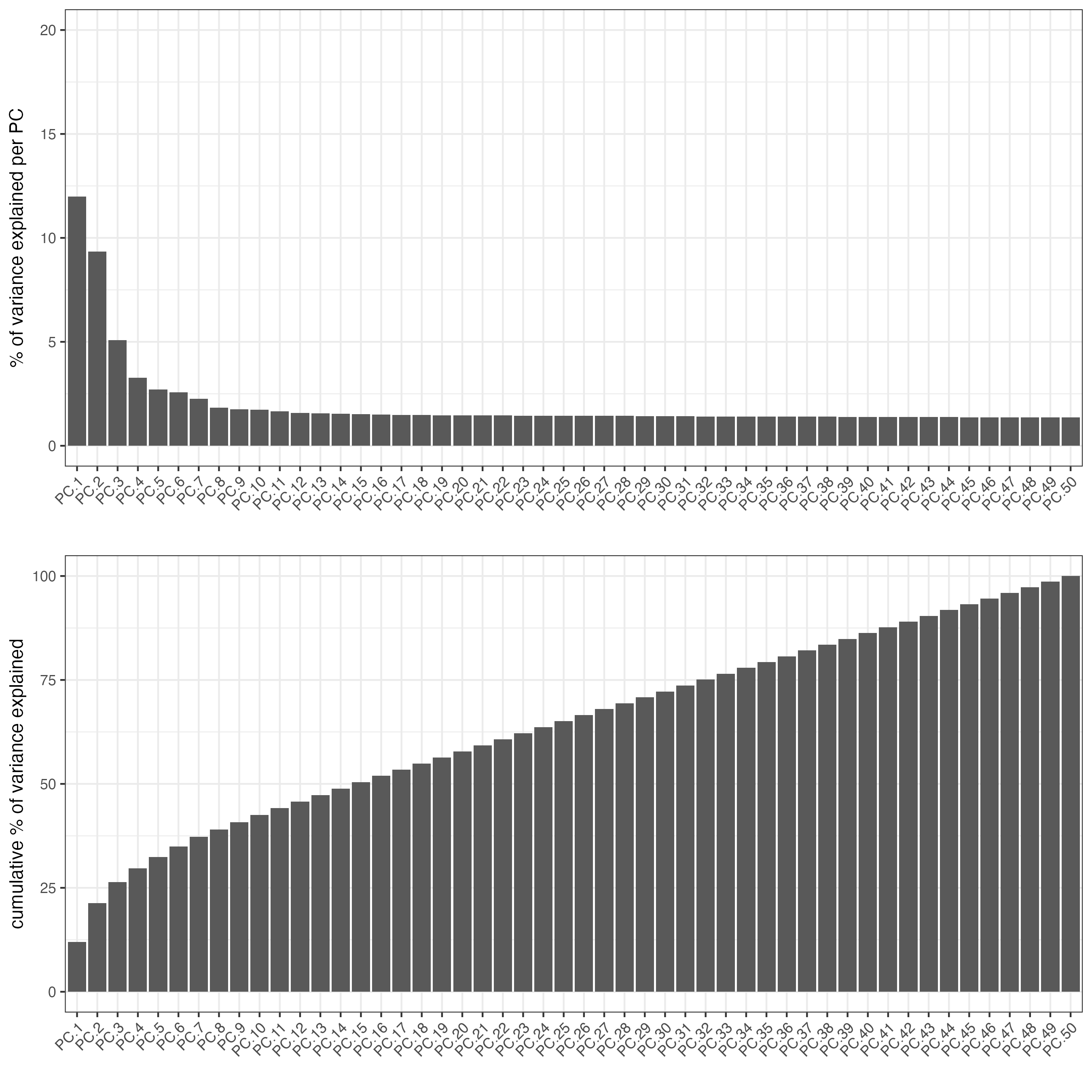
- Visualize the PCA calculated using the HVFs.
plotPCA(gobject = g_cell)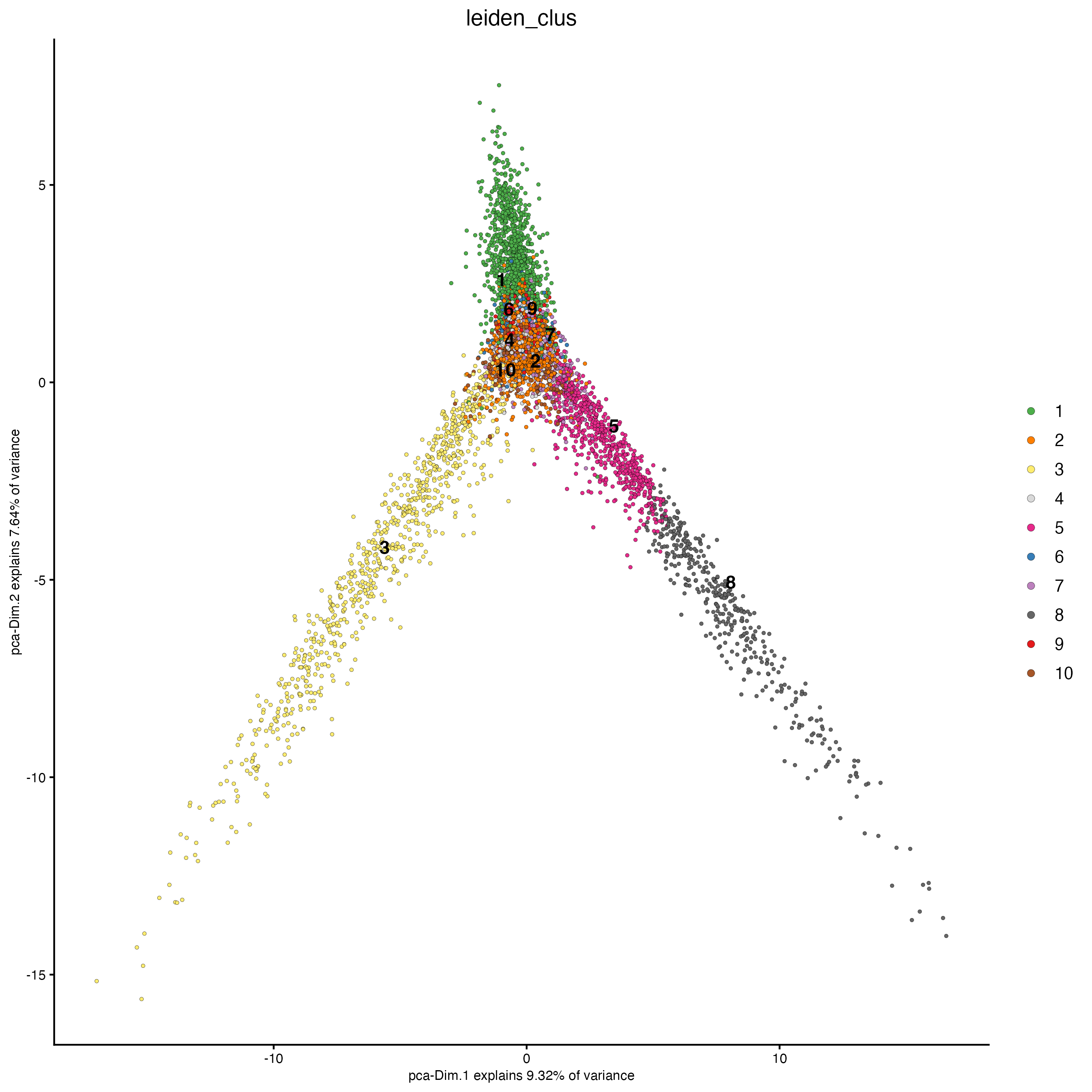
13.5.2 UMAP
Unlike PCA, Uniform Manifold Approximation and Projection (UMAP) and t-Stochastic Neighbor Embedding (t-SNE) do not assume linearity. After running PCA, UMAP or t-SNE allows you to visualize the dataset in 2D.
## run UMAP on PCA space (default)
g_cell <- runUMAP(g_cell,
                  dimensions_to_use = 1:10)

plotUMAP(gobject = g_cell)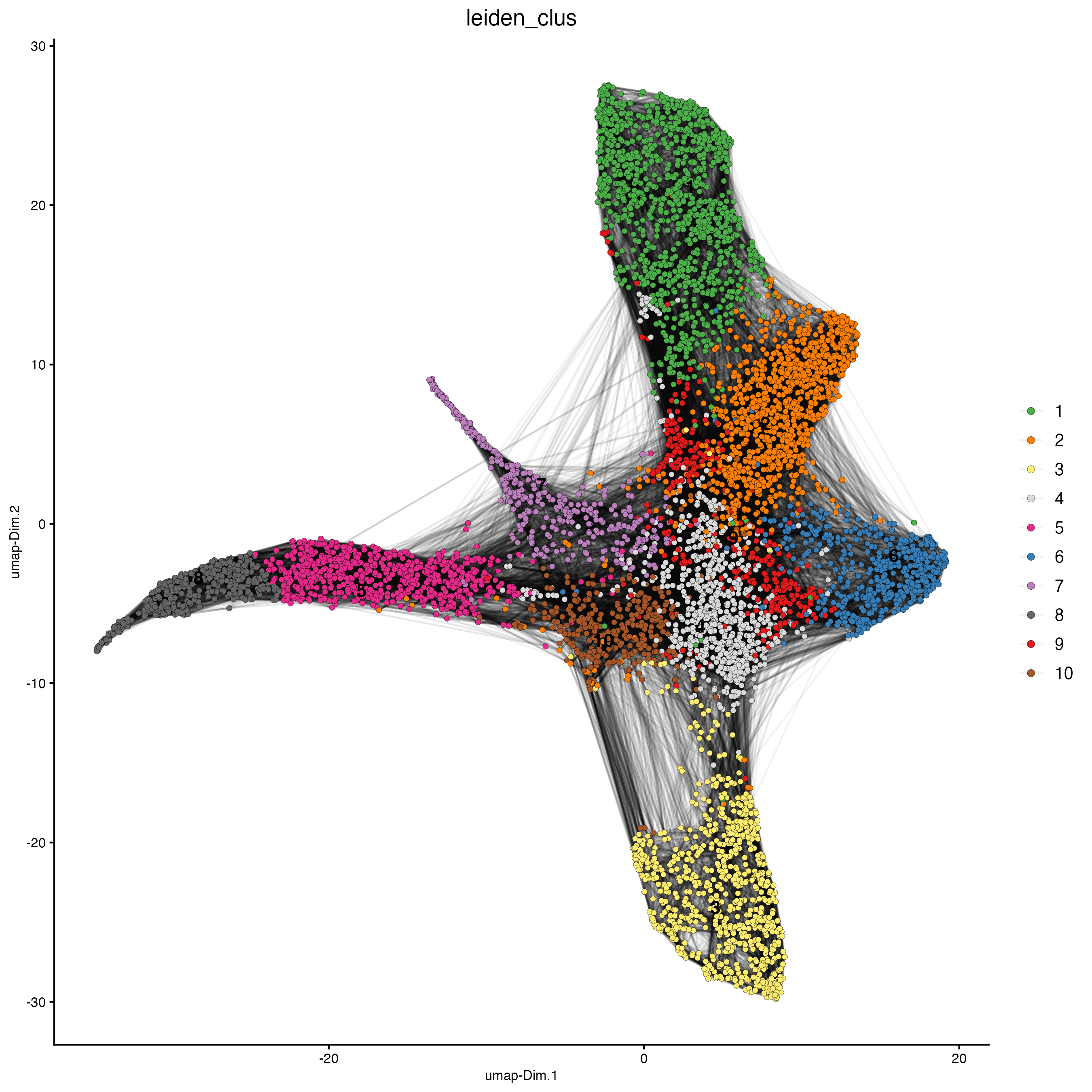
13.6 Clustering
13.6.1 Calculate the nearest neighbors
In preparation for the clustering calculation, finding the cells with similar expression patterns is needed. There are two methods available in Giotto:
- Create a sNN network (default)
The shared Nearest Neighbor algorithm defines the similarity between a pair of points in terms of their shared nearest neighbors. That is, the similarity between two points is “confirmed” by their common (shared) near neighbors. If point A is close to point B and if they are both close to a set of points C then we can say that A and B are close with greater confidence since their similarity is “confirmed” by the points in set C. You can find more information about this method here. By default, createNearestNetwork() calculates 30 shared Nearest Neighbors for each cell, but you can modify this number using the “k” parameter.
g_cell <- createNearestNetwork(gobject = g_cell,
dimensions_to_use = 1:10)- Create a kNN network
The K-Nearest Neighbors (kNN) algorithm operates on the principle of likelihood of similarity. It posits that similar data points tend to cluster near each other in space. You can find more information about this method here. By default, createNearestNetwork() finds the 30 K-Nearest Neighbors to each cell, but you can modify this number using the “k” parameter.
g_cell <- createNearestNetwork(gobject = g_cell,
                               dimensions_to_use = 1:10,
                               type = "kNN")
13.6.2 Leiden clustering
This algorithm is more complicated than the Louvain algorithm and have an accurate and fast result for the computation time. The Leiden algorithm consists of three phases. The first phase is the modularity optimization process, the second phase is the refinement of partition, and the third phase is the community aggregation process. This algorithm performs well on small, medium and large-scale networks. You can find more information about Louvain and Leiden clustering here
- Run the Leiden clustering algorithm.
g_cell <- doLeidenCluster(gobject = g_cell,
resolution = 1)- Plot dimension and spatial plots using the Leiden clusters information.
plotPCA(gobject = g_cell,
        cell_color = "leiden_clus")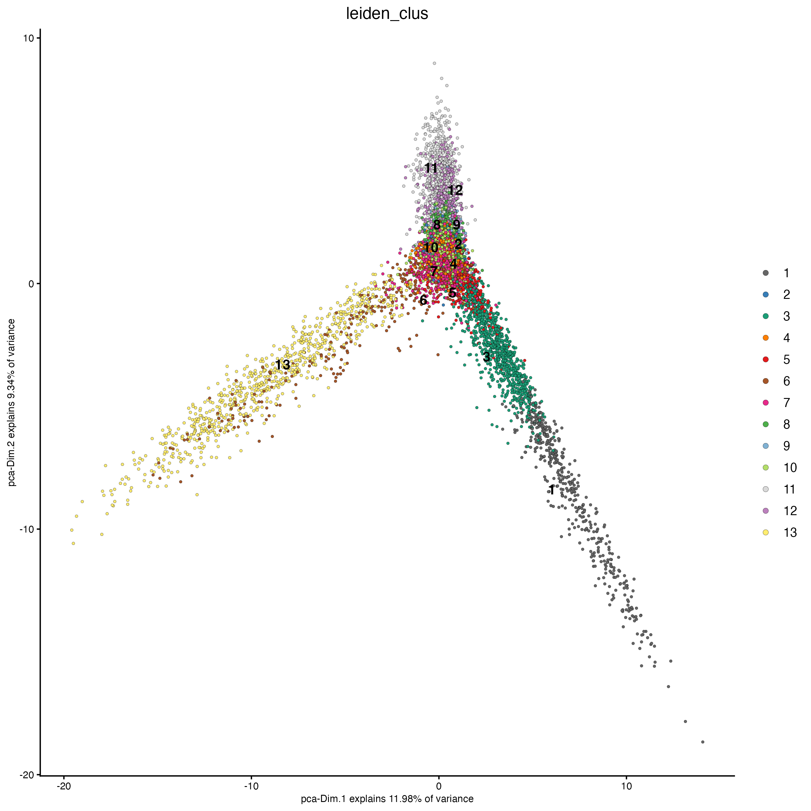
Set the argument “show_NN_network = TRUE” to visualize the connections between spots.
plotUMAP(gobject = g_cell,
         cell_color = "leiden_clus",
         show_NN_network = TRUE,
         point_size = 1.5)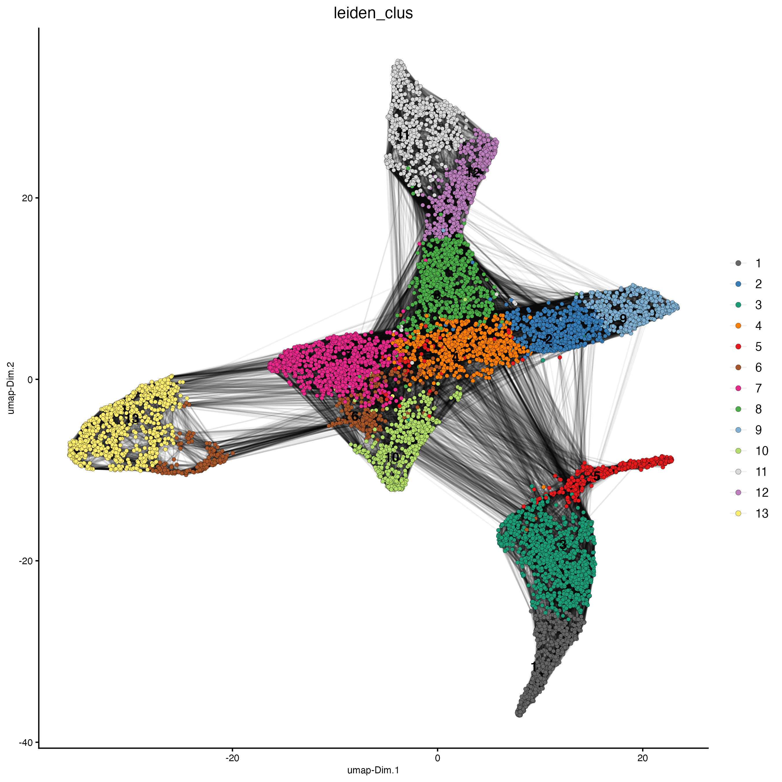
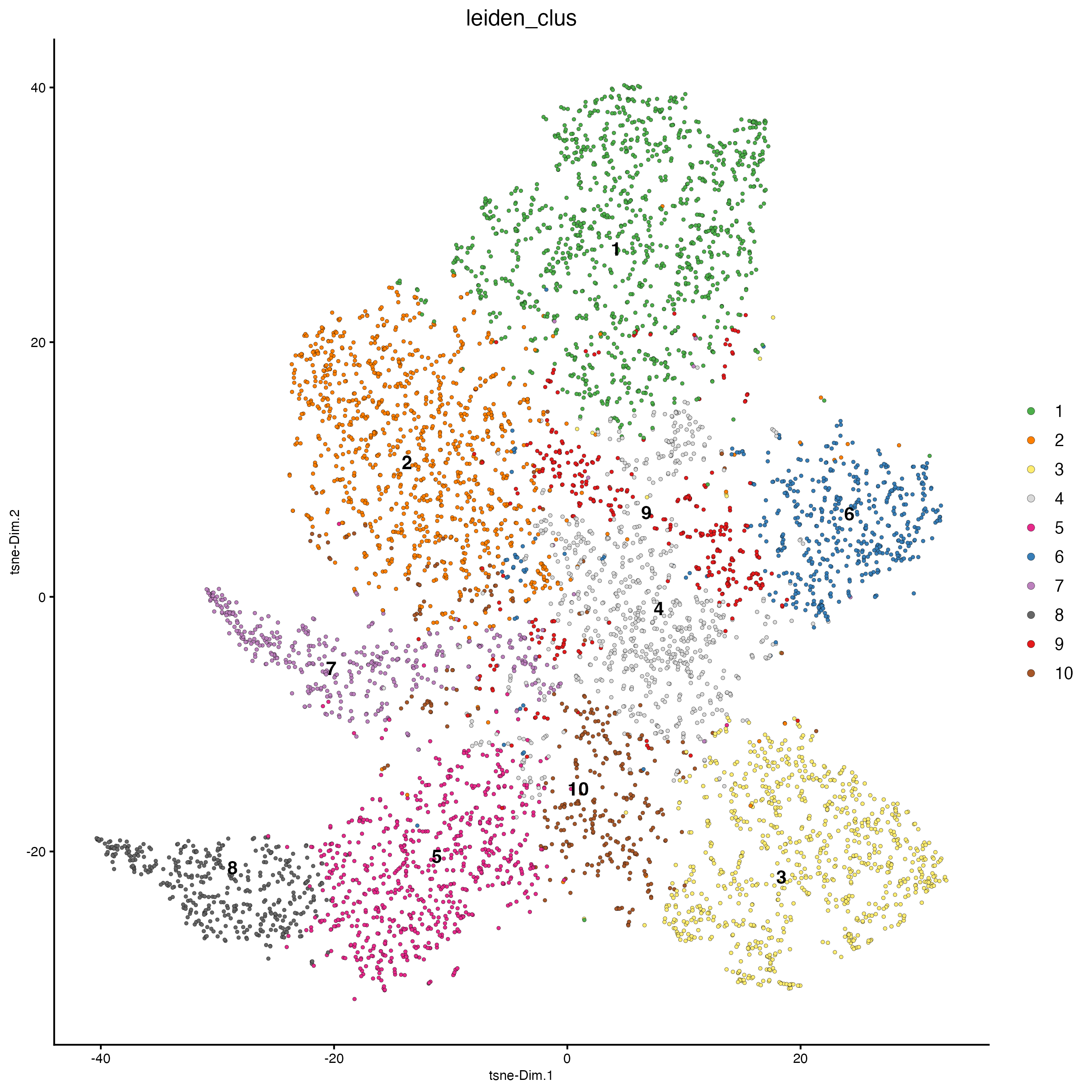
plotTSNE(gobject = g_cell,
         cell_color = "leiden_clus")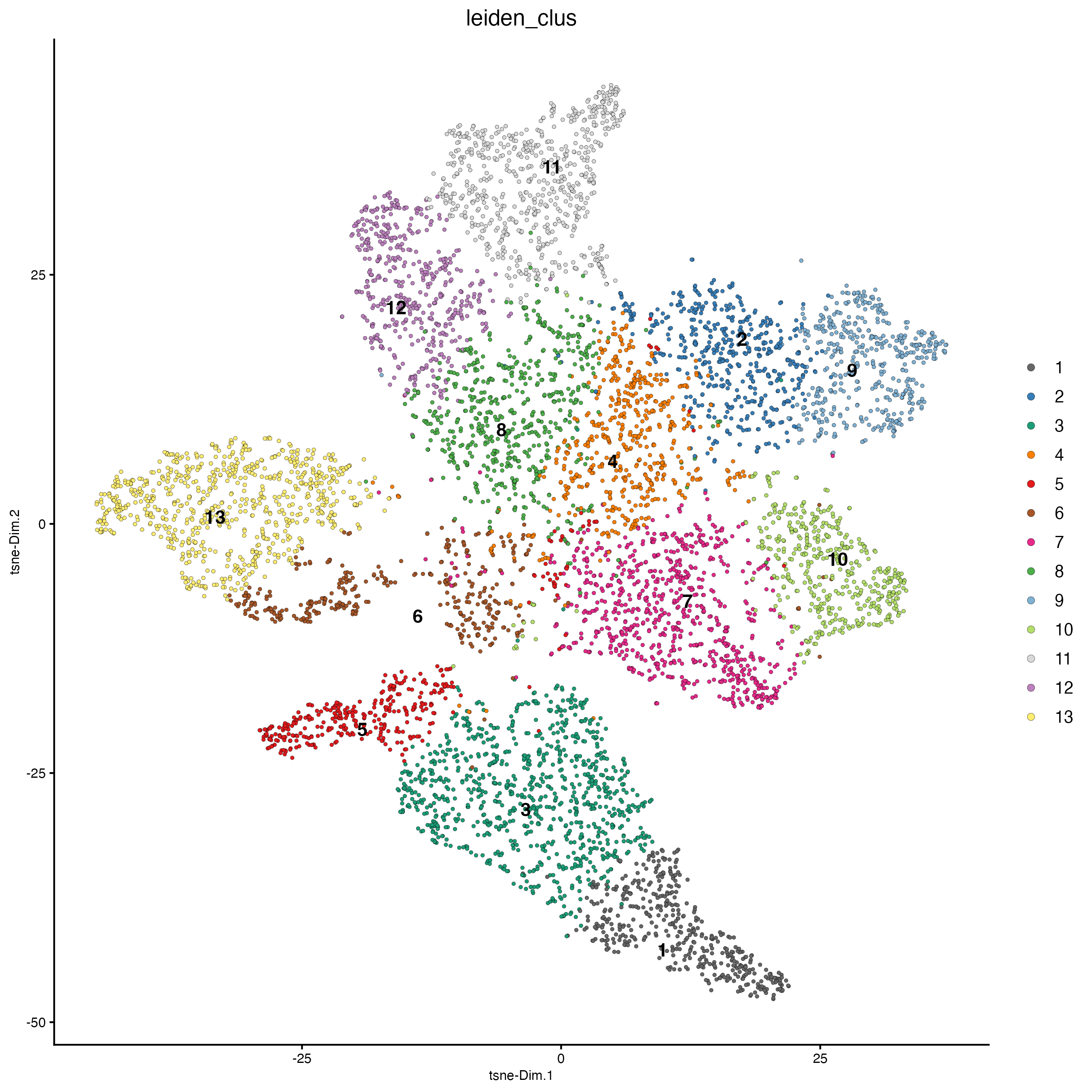
spatPlot2D(gobject = g_cell,
           point_size = 1,
           show_image = FALSE,
           background_color = "black",
           cell_color = "leiden_clus")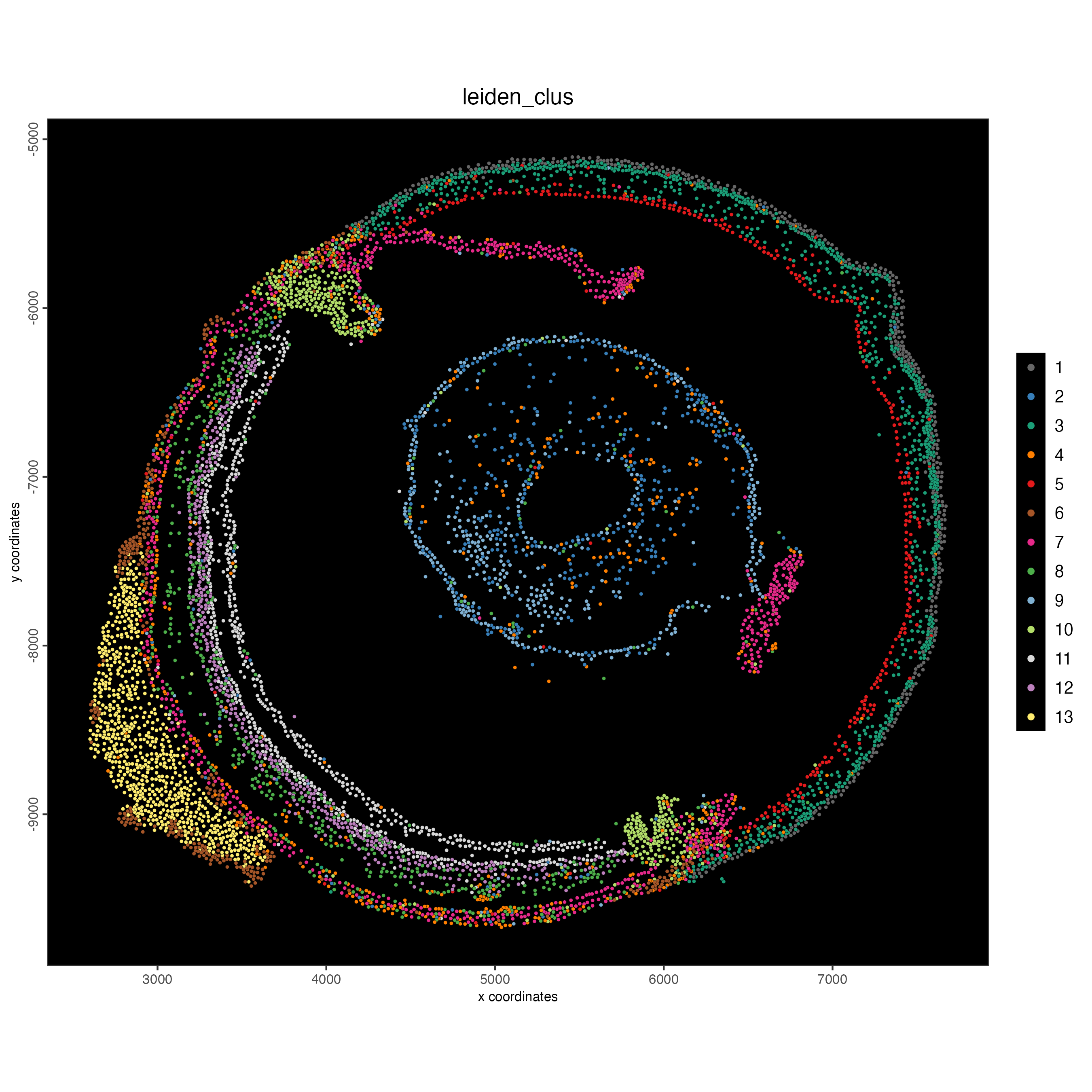
14 Process the Giotto object at the bin level
To follow this portion of the tutorial, use the bin100 object that only contains the features overlapping with the tissue. See the section “Read bin data using the convenience function”.
- Filtering
g_bin <- filterGiotto(gobject = g_bin,
                      expression_threshold = 1,
                      feat_det_in_min_cells = 10,
                      min_det_feats_per_cell = 50,
                      expression_values = "raw",
verbose = TRUE)- Normalization
g_bin <- normalizeGiotto(gobject = g_bin,
                         scalefactor = 6000,
verbose = TRUE)- Feature selection
g_bin <- calculateHVF(gobject = g_bin,
                      save_plot = TRUE)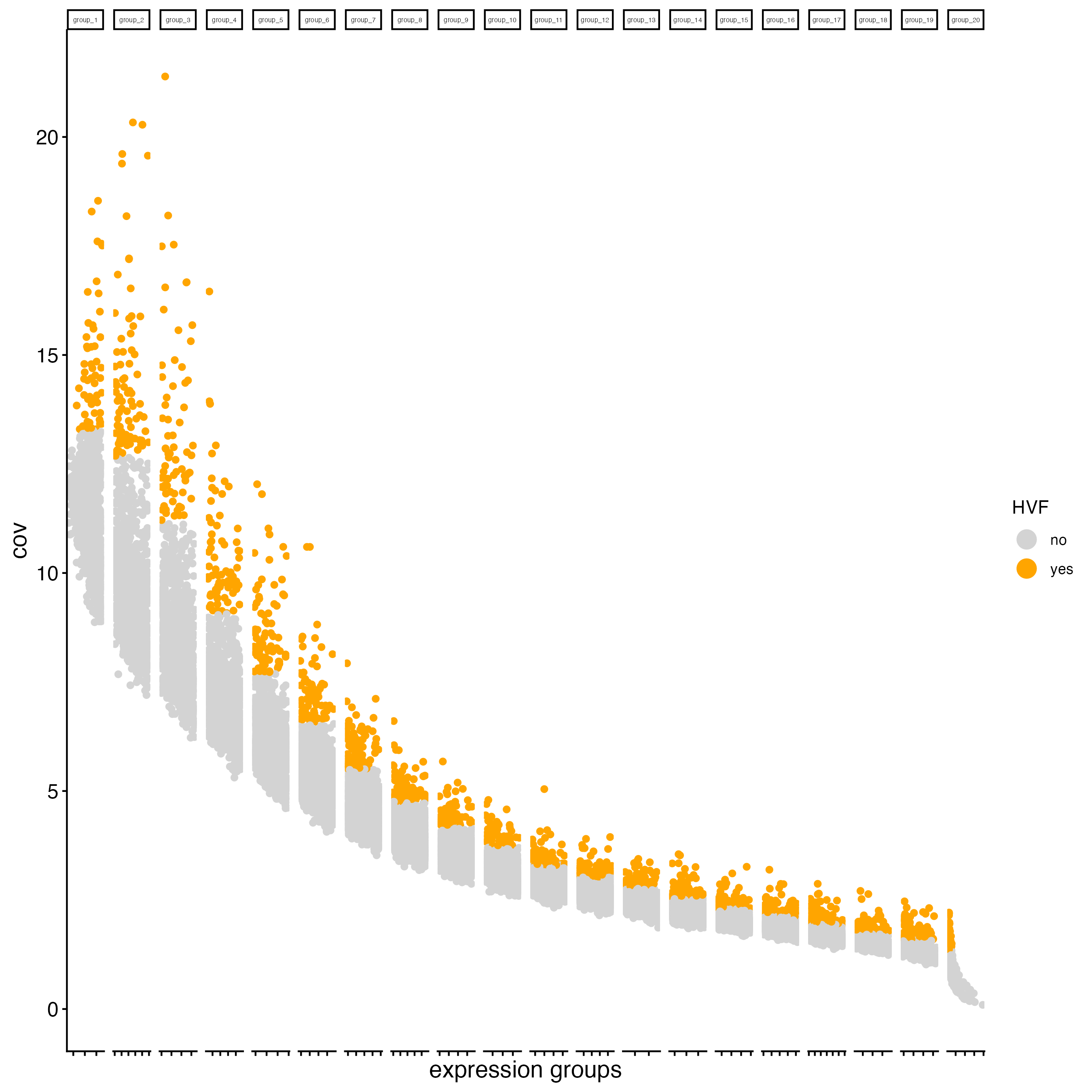
- Dimension reduction
g_bin <- runPCA(gobject = g_bin,
                ncp = 50)

g_bin <- runUMAP(g_bin,
                 dimensions_to_use = 1:10)

g_bin <- runtSNE(g_bin,
                 dimensions_to_use = 1:10,
check_duplicates = FALSE)- Create Nearest network
g_bin <- createNearestNetwork(gobject = g_bin,
dimensions_to_use = 1:10)- Run the Leiden clustering algorithm.
g_bin <- doLeidenCluster(gobject = g_bin,
                         resolution = 1)
plotUMAP(gobject = g_bin,
         cell_color = "leiden_clus",
         show_NN_network = TRUE,
         point_size = 1.5)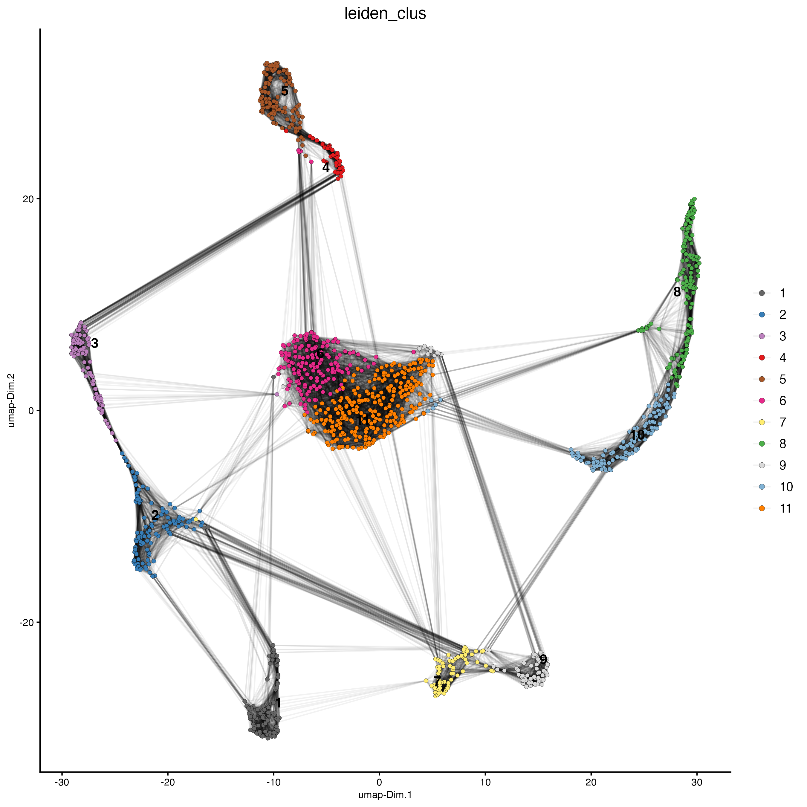
spatPlot2D(gobject = g_bin,
           point_size = 4,
           show_image = FALSE,
           point_alpha = 0.7,
           background_color = "black",
           cell_color = "leiden_clus")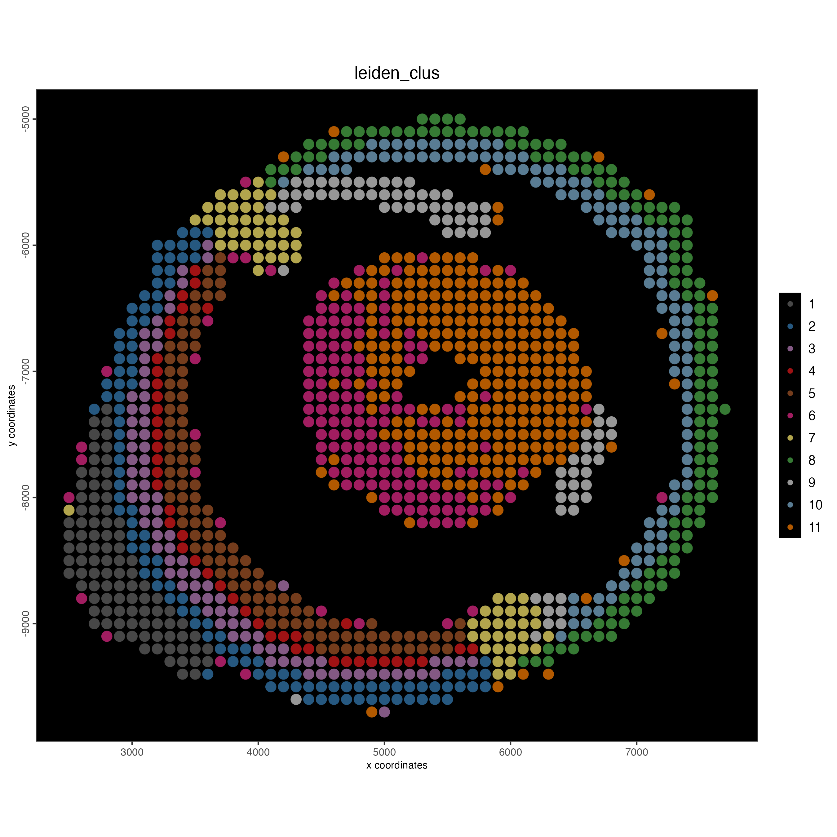
15 Session info
R version 4.5.3 (2026-03-11)
Platform: x86_64-apple-darwin20
Running under: macOS Tahoe 26.4.1

Matrix products: default
BLAS:   /System/Library/Frameworks/Accelerate.framework/Versions/A/Frameworks/vecLib.framework/Versions/A/libBLAS.dylib
LAPACK: /Library/Frameworks/R.framework/Versions/4.5-x86_64/Resources/lib/libRlapack.dylib;  LAPACK version 3.12.1

locale:
[1] en_US.UTF-8/en_US.UTF-8/en_US.UTF-8/C/en_US.UTF-8/en_US.UTF-8

time zone: America/New_York
tzcode source: internal

attached base packages:
[1] stats     graphics  grDevices utils     datasets  methods   base

other attached packages:
[1] Giotto_4.2.3      GiottoClass_0.5.1

loaded via a namespace (and not attached):
  [1] colorRamp2_0.1.0            gridExtra_2.3               remotes_2.5.0
  [4] rlang_1.2.0                 magrittr_2.0.5              RcppAnnoy_0.0.23
  [7] otel_0.2.0                  GiottoUtils_0.2.5           matrixStats_1.5.0
 [10] compiler_4.5.3              png_0.1-9                   systemfonts_1.3.2
 [13] vctrs_0.7.3                 pkgconfig_2.0.3             SpatialExperiment_1.20.0
 [16] fastmap_1.2.0               ellipsis_0.3.2              backports_1.5.1
 [19] magick_2.9.1                XVector_0.50.0              labeling_0.4.3
 [22] ggraph_2.2.2                sessioninfo_1.2.3           ragg_1.5.0
 [25] purrr_1.2.2                 xfun_0.57                   bluster_1.20.0
 [28] beachmat_2.26.0             cachem_1.1.0                jsonlite_2.0.0
 [31] rhdf5filters_1.22.0         DelayedArray_0.36.1         Rhdf5lib_1.32.0
 [34] BiocParallel_1.44.0         tweenr_2.0.3                terra_1.9-11
 [37] irlba_2.3.7                 parallel_4.5.3              cluster_2.1.8.2
 [40] R6_2.6.1                    RColorBrewer_1.1-3          reticulate_1.45.0
 [43] parallelly_1.47.0           pkgload_1.5.0               GenomicRanges_1.62.1
 [46] scattermore_1.2             Rcpp_1.1.1                  Seqinfo_1.0.0
 [49] SummarizedExperiment_1.40.0 knitr_1.51                  future.apply_1.20.2
 [52] usethis_3.2.1               R.utils_2.13.0              FNN_1.1.4.1
 [55] IRanges_2.44.0              Matrix_1.7-4                igraph_2.2.2
 [58] tidyselect_1.2.1            rstudioapi_0.18.0           abind_1.4-8
 [61] viridis_0.6.5               codetools_0.2-20            listenv_0.10.1
 [64] pkgbuild_1.4.8              lattice_0.22-9              tibble_3.3.1
 [67] Biobase_2.70.0              withr_3.0.2                 S7_0.2.1
 [70] Rtsne_0.17                  evaluate_1.0.5              future_1.70.0
 [73] polyclip_1.10-7             pillar_1.11.1               MatrixGenerics_1.22.0
 [76] checkmate_2.3.4             stats4_4.5.3                dbscan_1.2.4
 [79] plotly_4.12.0               generics_0.1.4              S4Vectors_0.48.0
 [82] ggplot2_4.0.2               sparseMatrixStats_1.22.0    scales_1.4.0
 [85] globals_0.19.1              gtools_3.9.5                glue_1.8.1
 [88] lazyeval_0.2.2              tools_4.5.3                 GiottoVisuals_0.2.14
 [91] BiocNeighbors_2.4.0         data.table_1.18.2.1         RSpectra_0.16-2
 [94] ScaledMatrix_1.18.0         fs_2.0.1                    graphlayouts_1.2.3
 [97] tidygraph_1.3.1             cowplot_1.2.0               rhdf5_2.54.1
[100] grid_4.5.3                  tidyr_1.3.2                 devtools_2.4.6
[103] colorspace_2.1-2            SingleCellExperiment_1.32.0 BiocSingular_1.26.1
[106] ggforce_0.5.0               rsvd_1.0.5                  cli_3.6.6
[109] textshaping_1.0.4           S4Arrays_1.10.1             viridisLite_0.4.3
[112] dplyr_1.2.1                 uwot_0.2.4                  gtable_0.3.6
[115] R.methodsS3_1.8.2           digest_0.6.39               BiocGenerics_0.56.0
[118] SparseArray_1.10.10         ggrepel_0.9.8               rjson_0.2.23
[121] htmlwidgets_1.6.4           farver_2.1.2                R.oo_1.27.1
[124] memoise_2.0.1               htmltools_0.5.9             lifecycle_1.0.5
[127] httr_1.4.8                  MASS_7.3-65