Whole transcriptome CosMx Human Pancreas FFPE Dataset
Source:vignettes/cosmx_pancreas.Rmd
cosmx_pancreas.Rmd1 Dataset explanation
CosMx Spatial Molecular Imager (SMI) was used to characterize human pancreas FFPE tissue with a 18,946 plex pre-commercial version of the CosMx Human Whole Transcriptome panel. This dataset was generated using a prototype version of the panel and related software.
More information about this dataset can be found here.
2 Download the dataset
Download the CosMx human pancreas FFPE dataset from here. Go to DOWNLOAD DATA > Basic Data Files. Once you have downloaded the .zip file, decompress the the file in your working directory.
3 Setup
Install the Giotto package and the Giotto environment.
# Ensure Giotto Suite is installed.
if(!"Giotto" %in% installed.packages()) {
  pak::pkg_install("drieslab/Giotto")
}

# Ensure the Python environment for Giotto has been installed.
genv_exists <- Giotto::checkGiottoEnvironment()
if(!genv_exists){
  # The following command need only be run once to install the Giotto environment.
  Giotto::installGiottoEnvironment()
}
Set the instructions to build the Giotto object and run the analysis.
library(Giotto)

# set working directory
results_folder <- "/path/to/results/"

# Optional: Specify a path to a Python executable within a conda or miniconda
# environment. If set to NULL (default), the Python executable within the previously
# installed Giotto environment will be used.
python_path <- NULL # alternatively, "/local/python/path/python" if desired.

## Set object behavior
# by directly saving plots, but not rendering them you will save a lot of time
instructions <- createGiottoInstructions(
    save_dir = results_folder,
    save_plot = TRUE,
    show_plot = FALSE,
    return_plot = FALSE,
    python_path = python_path
)

## provide the path to "Pancreas-CosMx-WTx-FlatFiles" folder.
data_path <- "/path/to/data/"
4 Create the Giotto object using the provided aggregated expression matrix
You can create the object using the expression file that contains the pre-aggregated features.
cosmx <- createGiottoCosMxObject(
    cosmx_dir = data_path,
    version = "default",
    load_expression = TRUE,
    load_transcripts = FALSE,
    feat_type = c("rna", "SystemControl"),
    split_keyword = list("SystemControl"),
    instructions = instructions
)
5 Create the Giotto object using the subcellular information
Alternatively, you can create the object using the transcripts file and then aggregate the features per polygon/cell in a step below.
cosmx <- createGiottoCosMxObject(
    cosmx_dir = data_path,
    version = "default",
    load_expression = FALSE,
    load_transcripts = TRUE,
    feat_type = c("rna", "SystemControl"),
    split_keyword = list("SystemControl"),
    instructions = instructions
)
CosMx data is very FOV-based, and a column called fov is
included in the cell metadata.
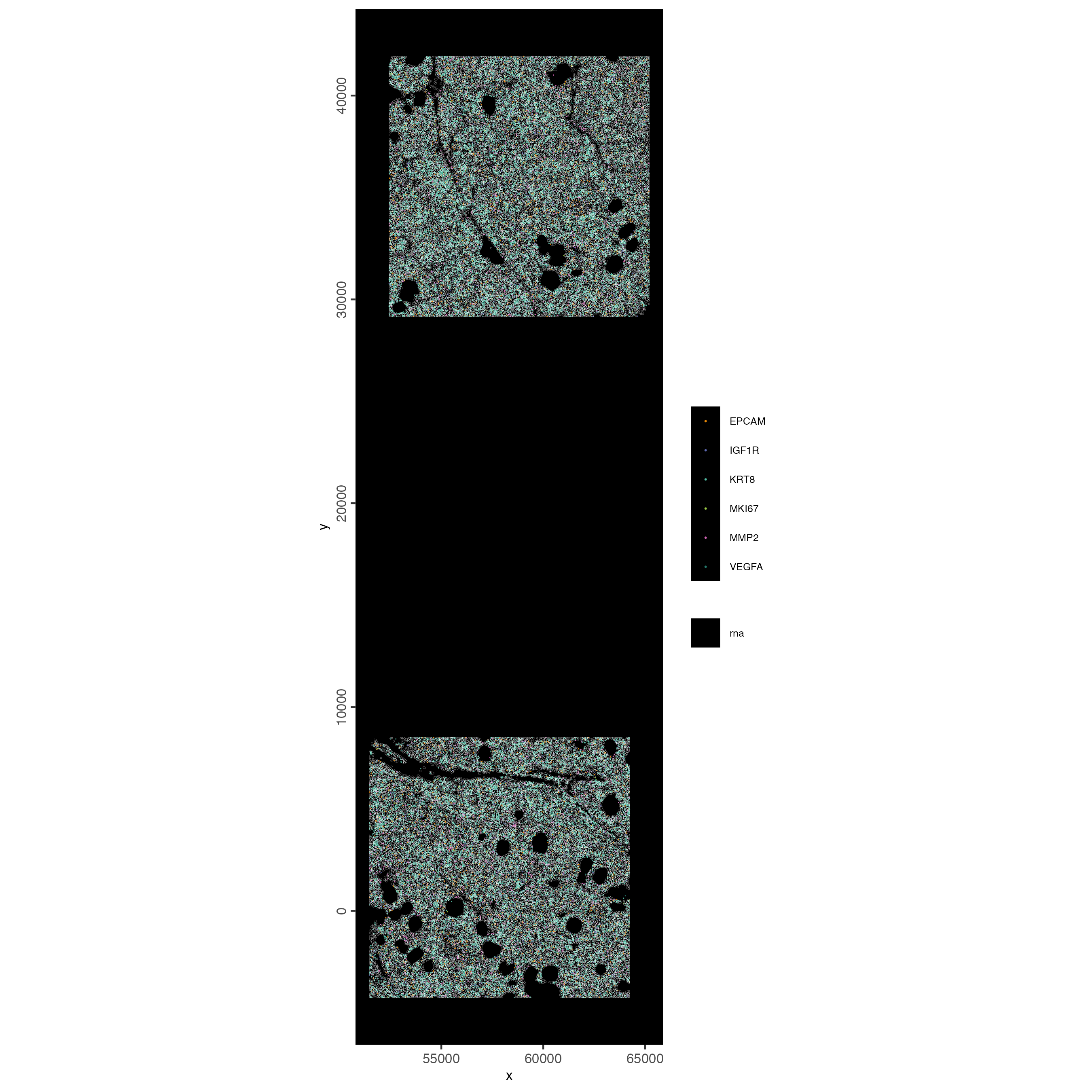
6 Visualize Cells and Genes of Interest
When plotting subcellular data, Giotto uses the
spatInSituPlot functions. Spatial plots showing the feature
points and polygons are plotted using
spatInSituPlotPoints().
spatInSituPlotPoints(cosmx,
    show_image = FALSE,
    feats = list("rna" = c(
        "MMP2", "VEGFA", "IGF1R",
        "MKI67", "EPCAM", "KRT8")
        ),
    feats_color_code = getColors("Vivid", 10),
    spat_unit = "cell",
    point_size = 0.01,
    use_overlap = FALSE,
    polygon_alpha = 0,
    polygon_color = "white",
    polygon_line_size = 0.03
)
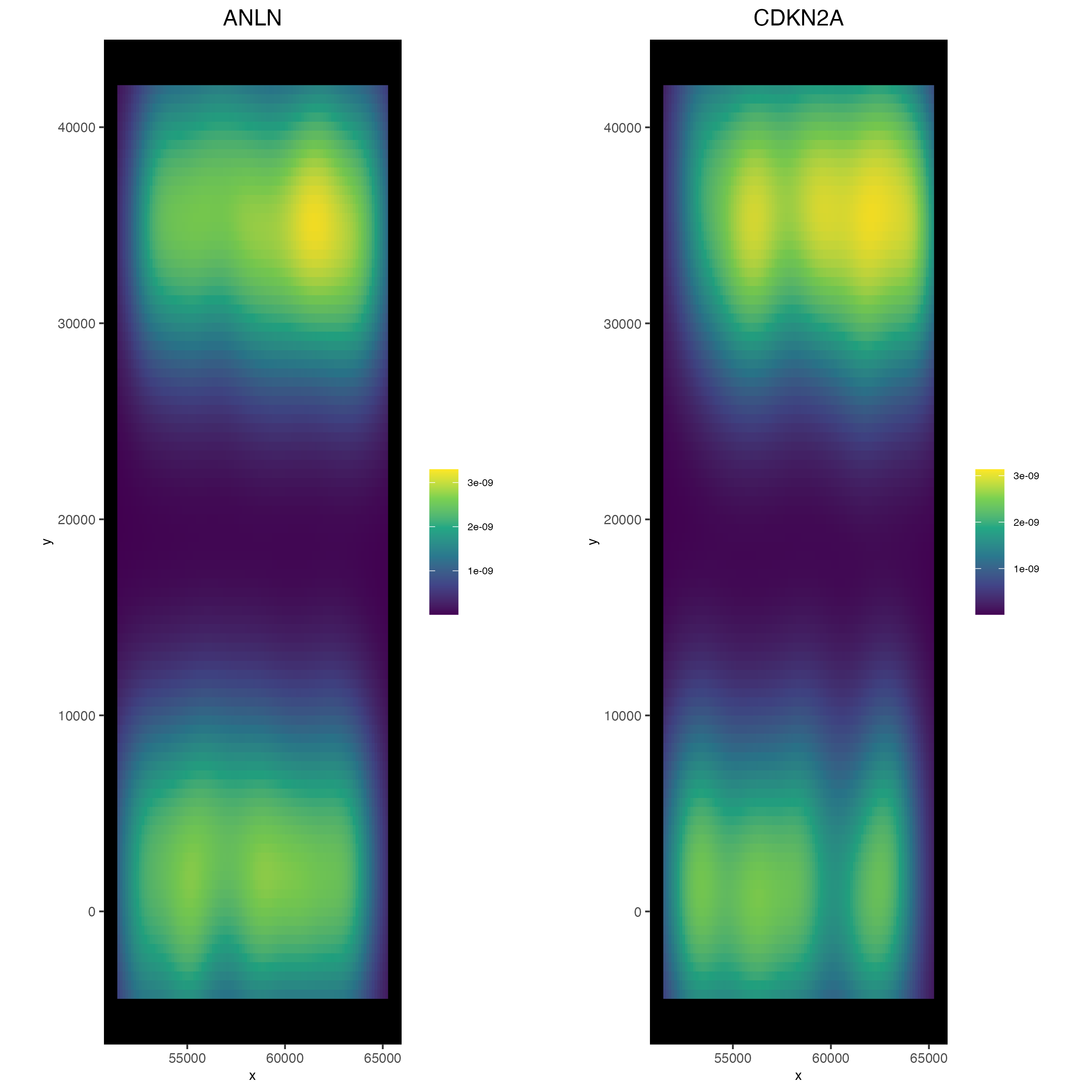
6.1 2D Density Plots
Density-based representations may sometimes be preferred instead of viewing the raw points information, especially when points are dense enough that there is overplotting.
spatInSituPlotDensity(cosmx,
    show_polygon = FALSE,
    use_overlap = FALSE,
    feats = c("ANLN", "CDKN2A"),
    cow_n_col = 2
)
7 Aggregate subcellular features
For more information on feature aggregation, click here
To generate a cell by feature matrix, Giotto performs feature detection aggregation based on the cell polygons. This workflow is recommended over loading the matrix provided in the outputs.
If directly loading the expression info in the outputs is desired,
set load_expression (and also load_cellmeta)
to TRUE when creating the object with
createGiottoCosMxObject()
# Find the feature points overlapped by polygons and convert the overlap
# information into a cell by feature expression matrix which
# is then stored in the Giotto object's expression slot
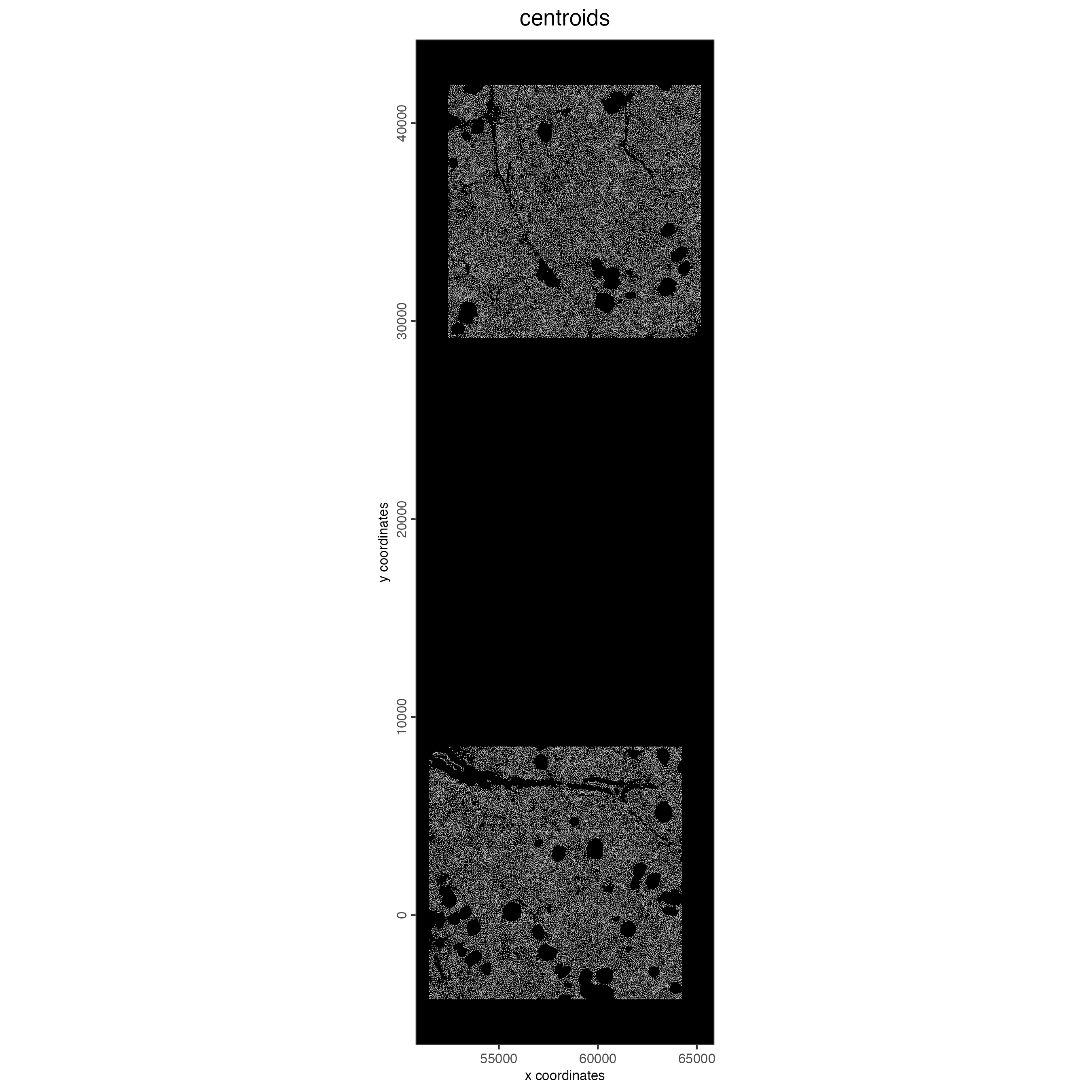
cosmx <- aggregateFeatures(cosmx, feat_info = "rna")7.1 Visualize Cell Centroids
spatPlot2D(cosmx,
    show_image = FALSE,
    point_border_stroke = 0,
    background_color = "black",
    cell_color = "white",
    point_size = 0.3,
    point_alpha = 0.8,
    title = "centroids"
)
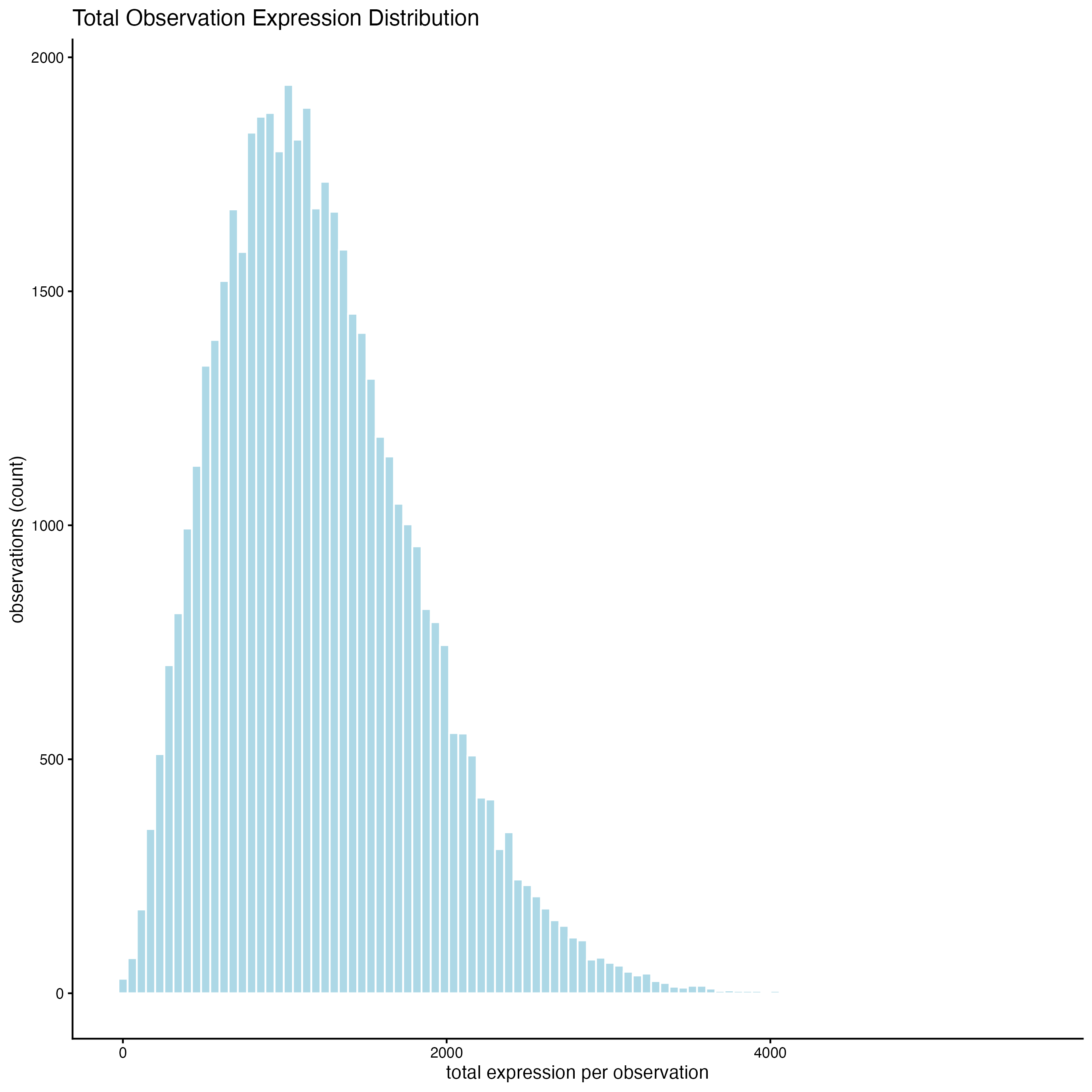
7.2 Plot histograms of total counts per cell
filterDistributions(cosmx,
    plot_type = "hist",
    detection = "cells",
    method = "sum",
    feat_type = "rna",
    nr_bins = 100
)
8 Filtering
cosmx <- filterGiotto(cosmx,
    feat_type = "rna",
    expression_threshold = 1,
    feat_det_in_min_cells = 100,
    min_det_feats_per_cell = 100
)
9 Normalization
- standard normalization method: library size normalization and log normalization. This method will produce both normalized and scaled values that are be returned as the “normalized” and “scaled”expression matrices respectively. In this tutorial, the normalized values will be used for generating expression statistics and plotting expression values. The scaled values will be ignored. We will also generate normalized values for the negative probes for visualization purposes during which the library normalization step will be skipped.
# For the purpose of running this tutorial in a fast an low-memory way, we will skip the scaling of cells and features. If you prefer to keep the scaling calculations, set scale_feats = TRUE, and scale_cells = TRUE (default values).
cosmx <- normalizeGiotto(cosmx,
    feat_type = "rna",
    norm_methods = "standard",
    scale_feats = FALSE,
    scale_cells = FALSE
)- pearson residuals: A normalization that uses the method described in Lause/Kobak et al, 2021. This produces a set of values that are most similar in utility to a scaled matrix and offer improvements to both HVF detection and PCA generation. These values should not be used for statistics, plotting of expression values, or differential expression analysis.
cosmx <- normalizeGiotto(cosmx,
    feat_type = "rna",
    norm_methods = "pearson_resid",
    name = "pearson",
    scale_feats = FALSE,
    scale_cells = FALSE
)
# add statistics based on log normalized values
cosmx <- addStatistics(cosmx,
    expression_values = "normalized",
    feat_type = "rna"
)

# View cellular data (default is feat = "rna")
showGiottoCellMetadata(cosmx)

# View feature data
showGiottoFeatMetadata(cosmx)
Note: The show functions for metadata do not return
the information. To retrieve the metadata information, instead use
pDataDT() and fDataDT() along with the
feat_type param for either “rna” or “negprobes”.
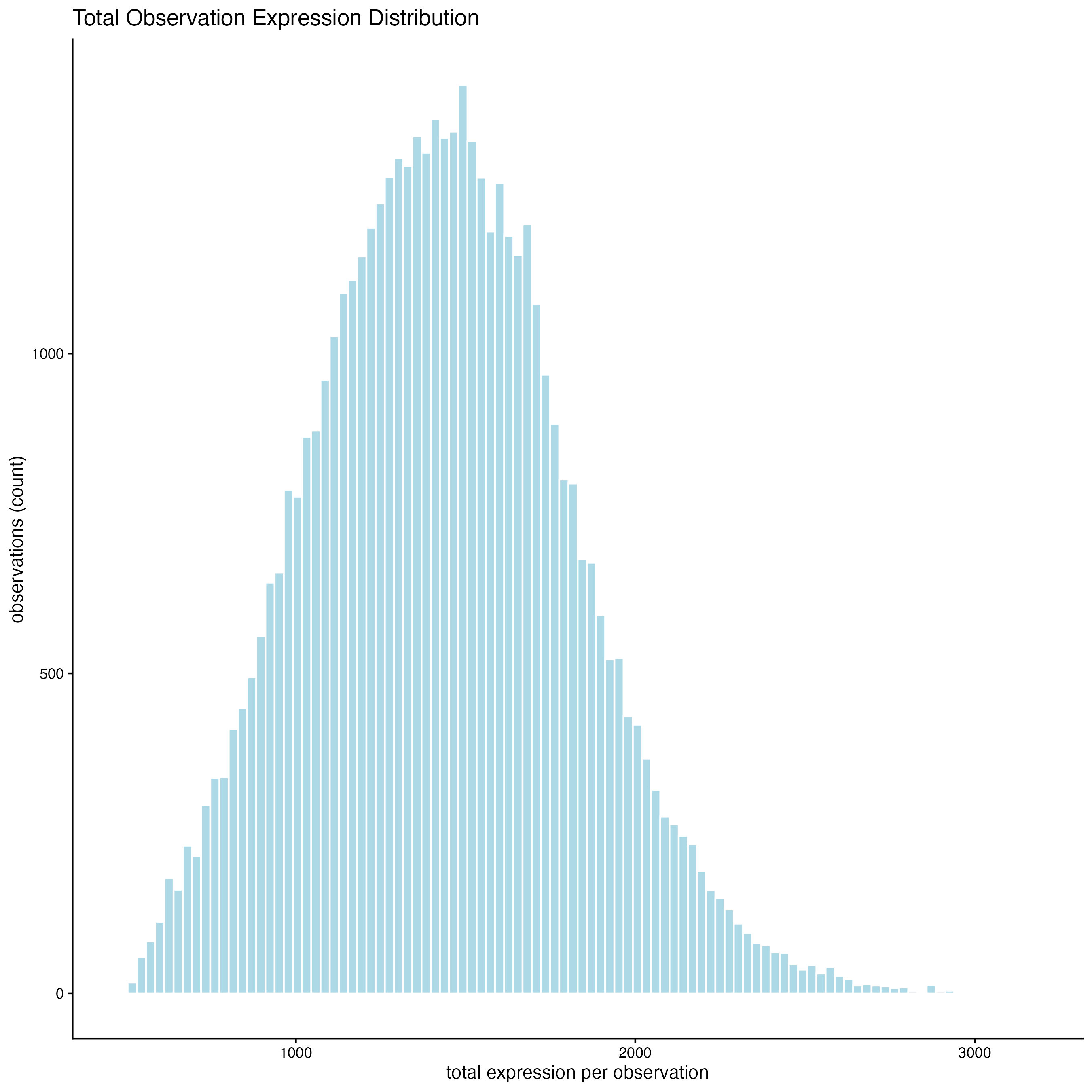
10 View Transcript Total Expression Distribution
10.1 Histogram of log normalized data
filterDistributions(cosmx,
    detection = "cells",
    feat_type = "rna",
    expression_values = "normalized",
    method = "sum",
    nr_bins = 100
)
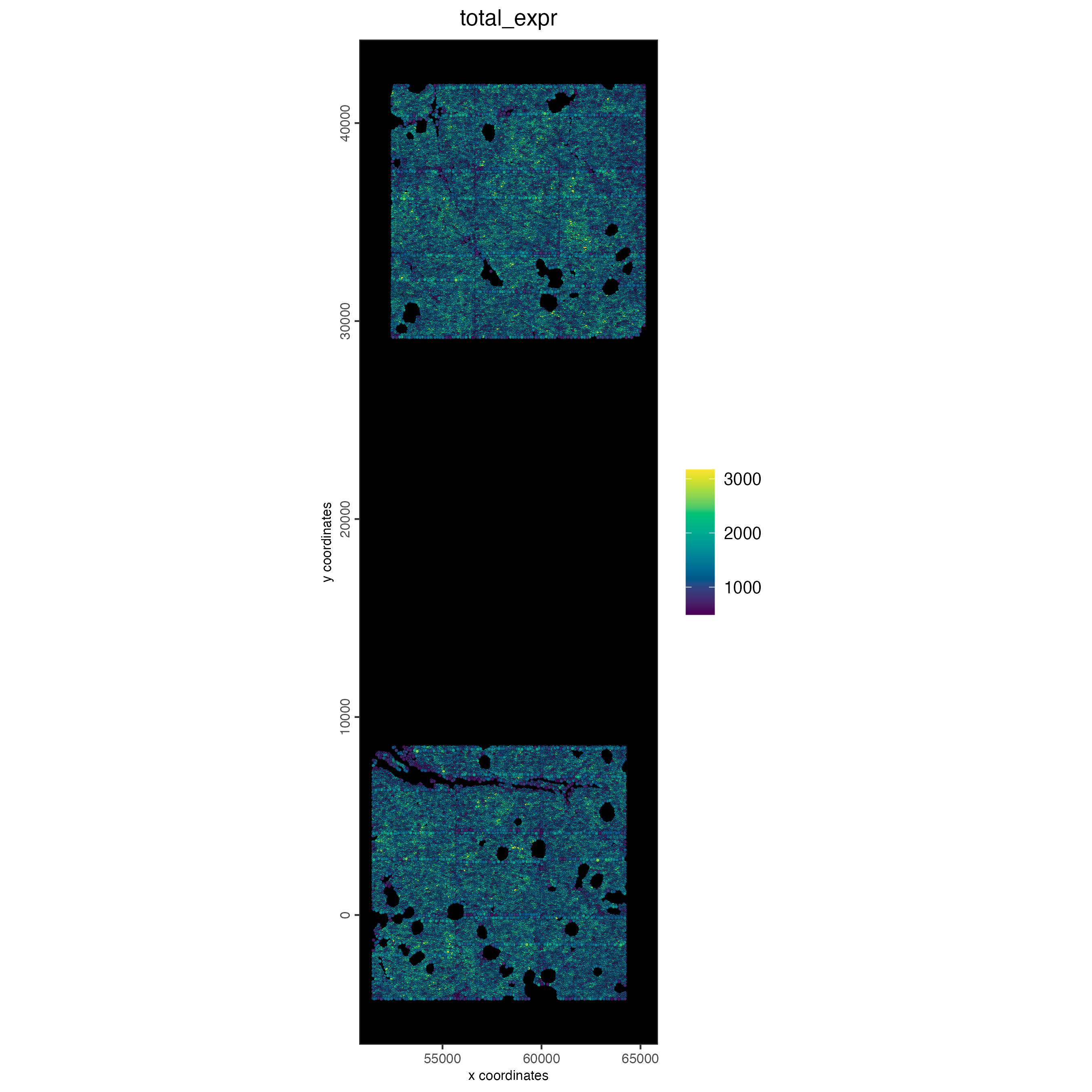
10.2 Plot normalized total expression
spatPlot2D(cosmx,
    cell_color = "total_expr",
    gradient_style = "sequential",
    color_as_factor = FALSE,
    point_size = 0.9,
    background_color = "black"
)
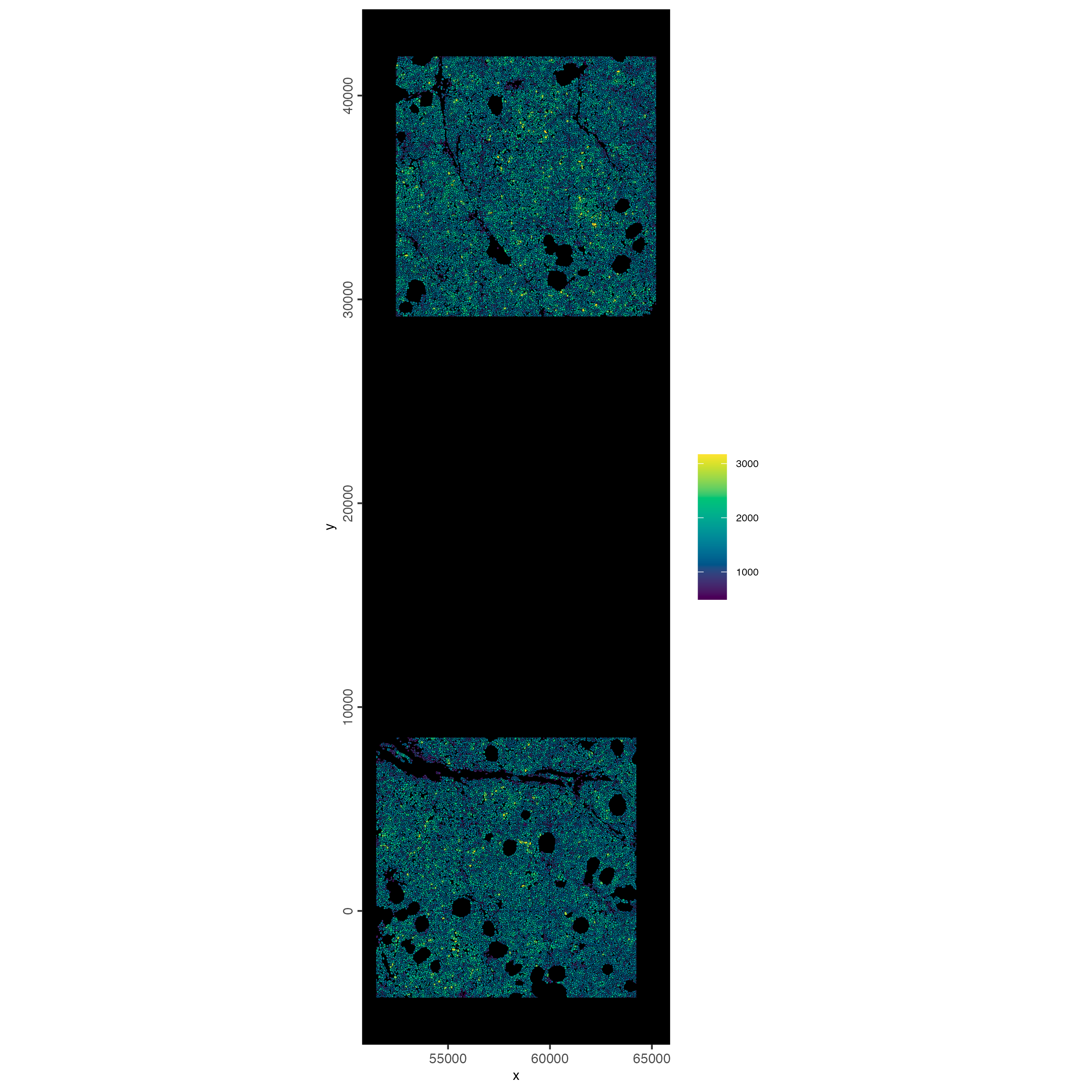
10.3 Plot spatially as color-scaled polygons
spatInSituPlotPoints(cosmx,
    show_polygon = TRUE,
    polygon_fill_gradient_style = "sequential",
    polygon_color = "black",
    polygon_line_size = 0.05,
    polygon_fill = "total_expr",
    polygon_fill_as_factor = FALSE
)
11 Dimension Reduction
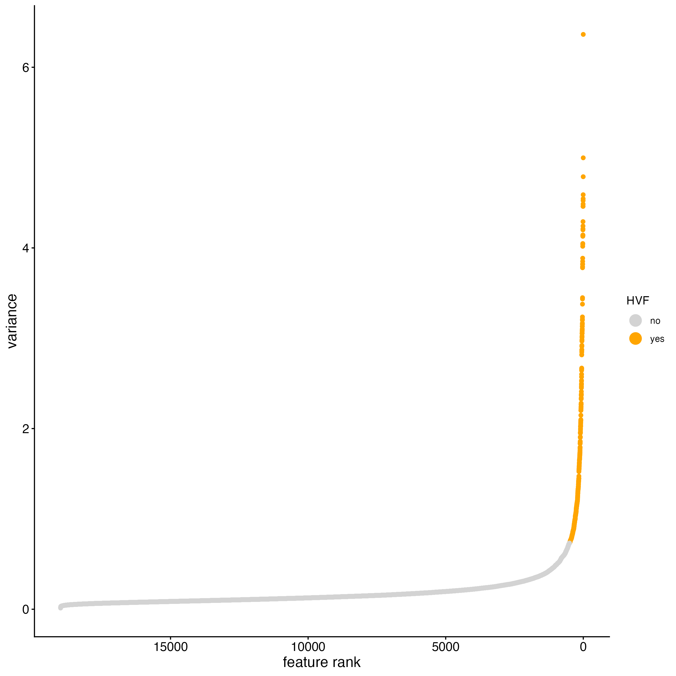
11.1 Detect highly variable genes and generate PCA
Detect highly variable genes using the pearson residuals method based on the “pearson” expression matrix. These results will be returned in the “hvf” column in the “rna” feature metadata.
cosmx <- calculateHVF(cosmx,
    method = "var_p_resid",
    var_number = 500, # leaving as NULL results in too few genes to use
    save_plot = TRUE
)
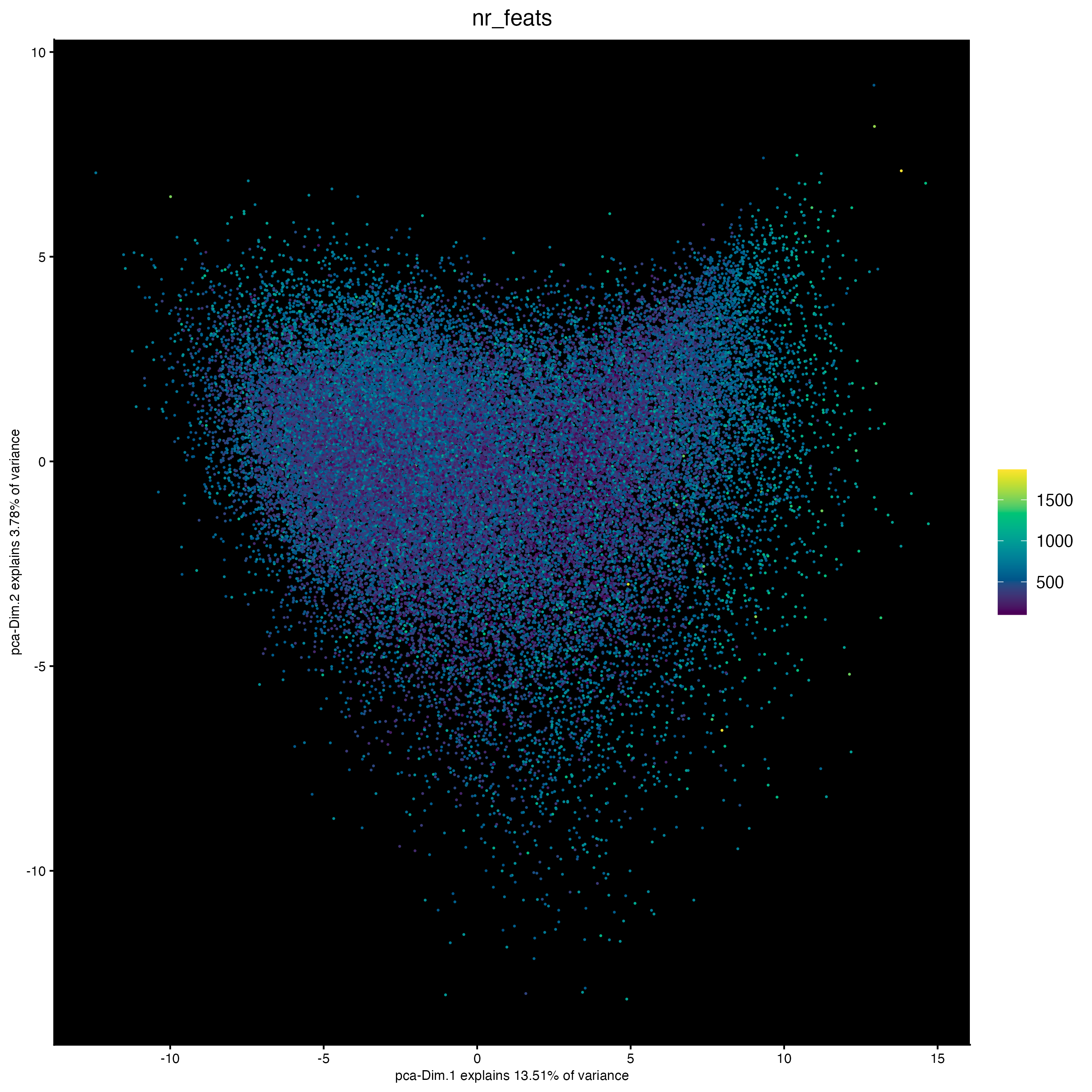
PCA generation will also be based on the “pearson” matrix. Scaling and centering of the PCA which is usually done by default will be skipped since the pearson matrix is already scaled.
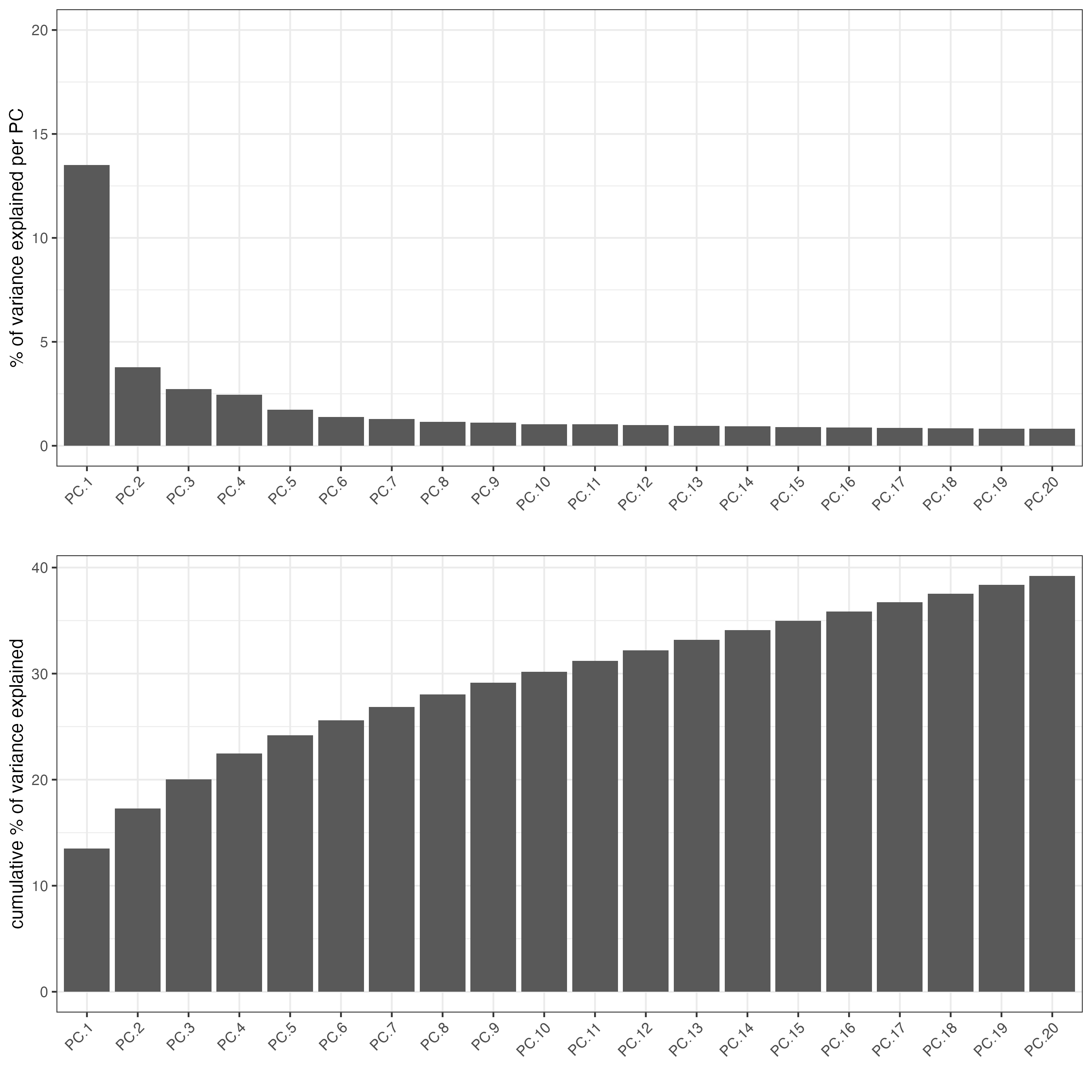
plotPCA(cosmx,
    cell_color = "nr_feats", # (from log norm expression statistics)
    color_as_factor = FALSE,
    point_size = 0.8,
    gradient_style = "sequential",
    point_border_stroke = 0,
    background_color = "black"
)
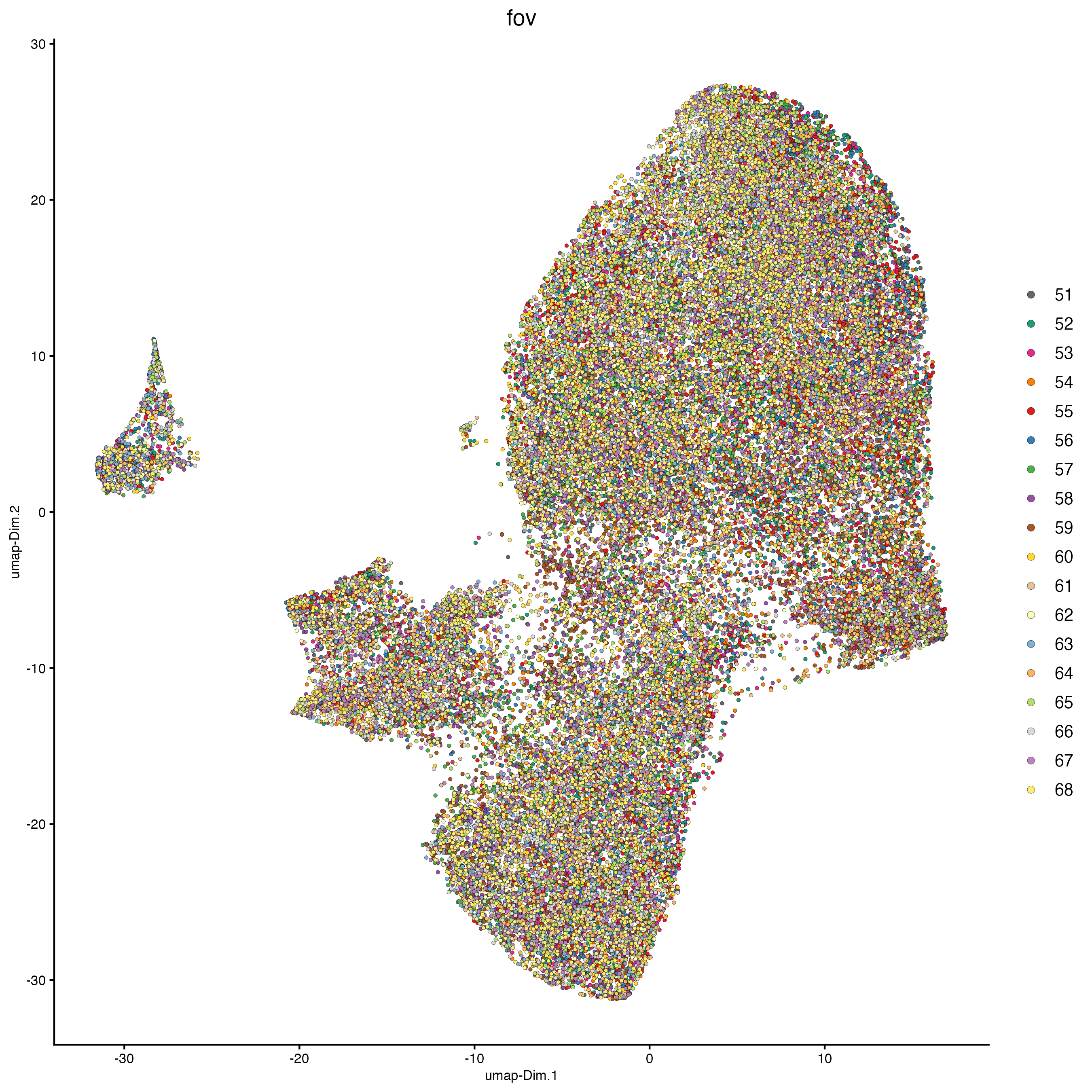
11.2 Run tSNE and UMAP
plotUMAP(cosmx,
         cell_color = "fov",
         show_center_label = FALSE
)
plotTSNE(cosmx,
         cell_color = "fov",
         show_center_label = FALSE
)

showGiottoDimRed(cosmx)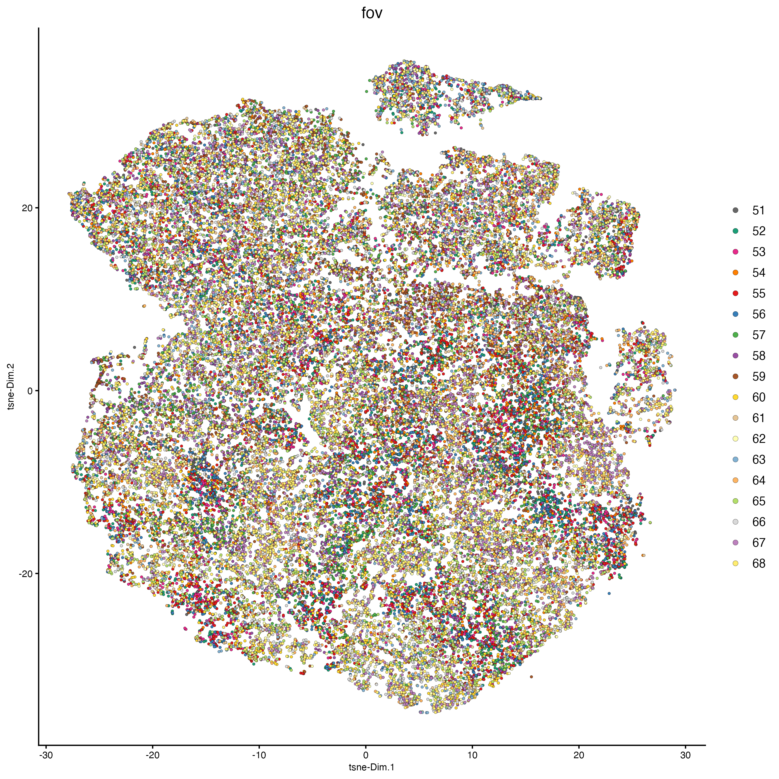
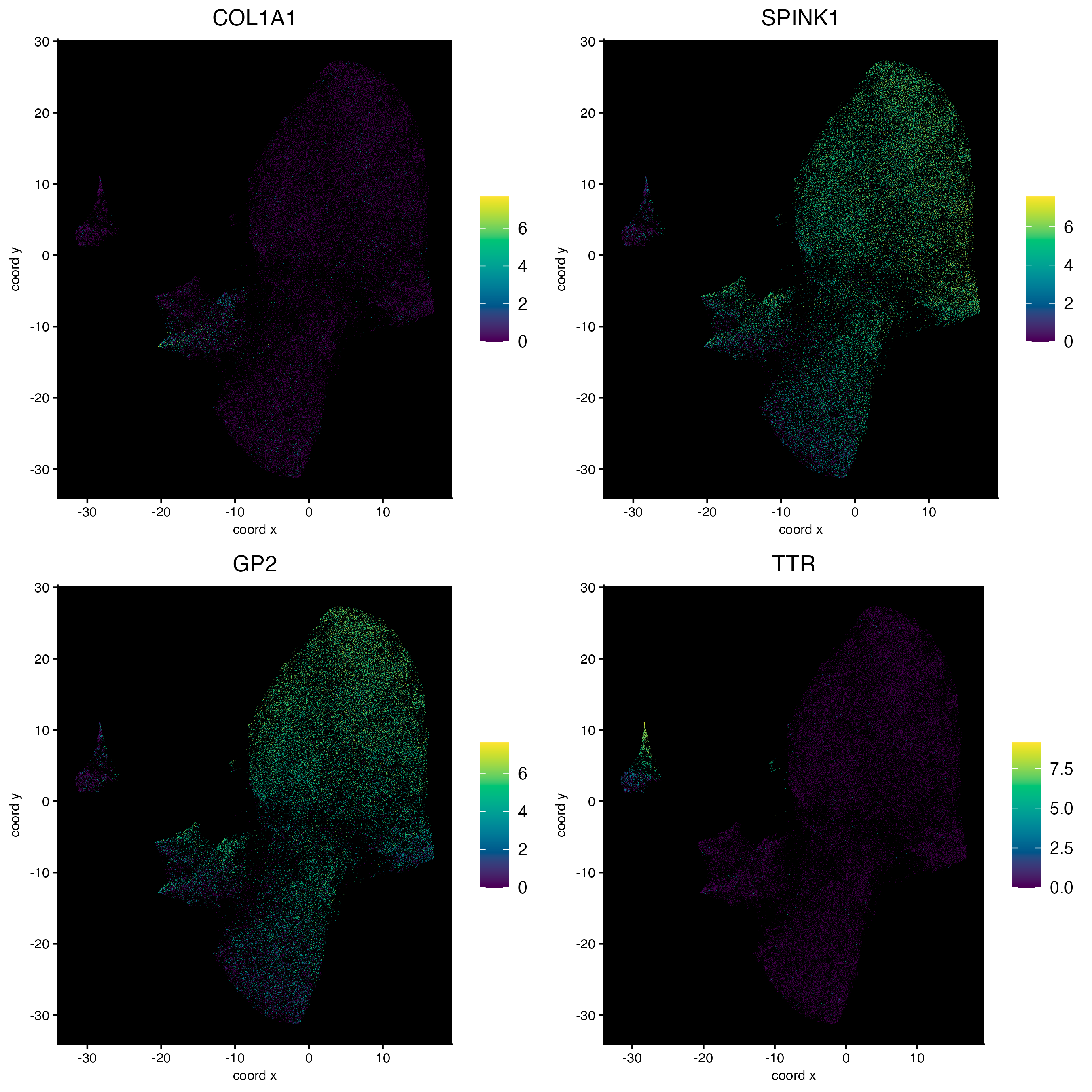
11.3 Plot features on expression space
dimFeatPlot2D(cosmx,
    feats = c("COL1A1", "SPINK1", "GP2", "TTR"),
    expression_values = "normalized",
    gradient_style = "sequential",
    point_border_stroke = 0,
    point_size = 0.2,
    cow_n_col = 2,
    background_color = "black"
)
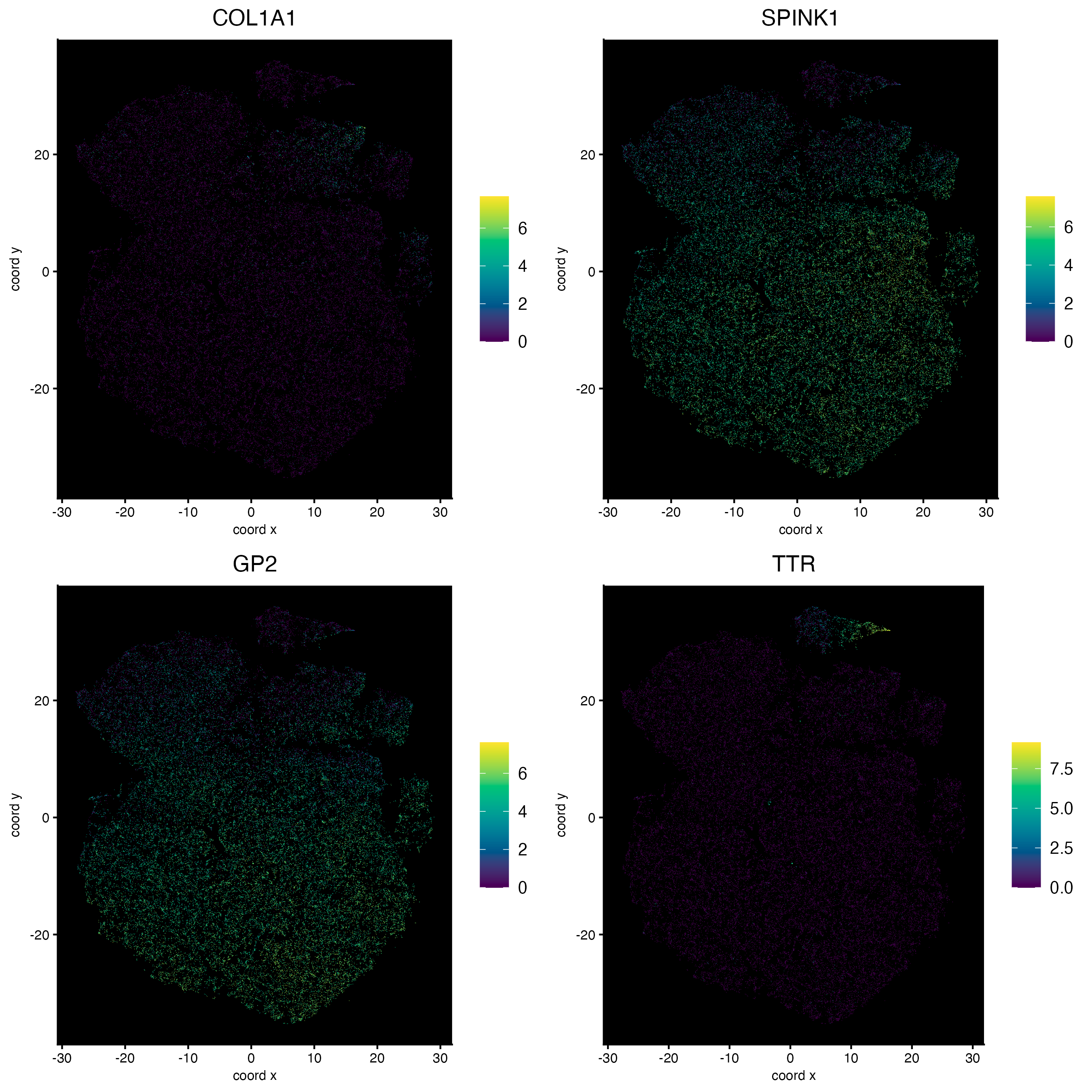
dimFeatPlot2D(cosmx,
    feats = c("COL1A1", "SPINK1", "GP2", "TTR"),
    expression_values = "normalized",
    dim_reduction_to_use = "tsne",
    dim_reduction_name = "tsne",
    gradient_style = "sequential",
    point_border_stroke = 0,
    point_size = 0.2,
    cow_n_col = 2,
    background_color = "black"
)
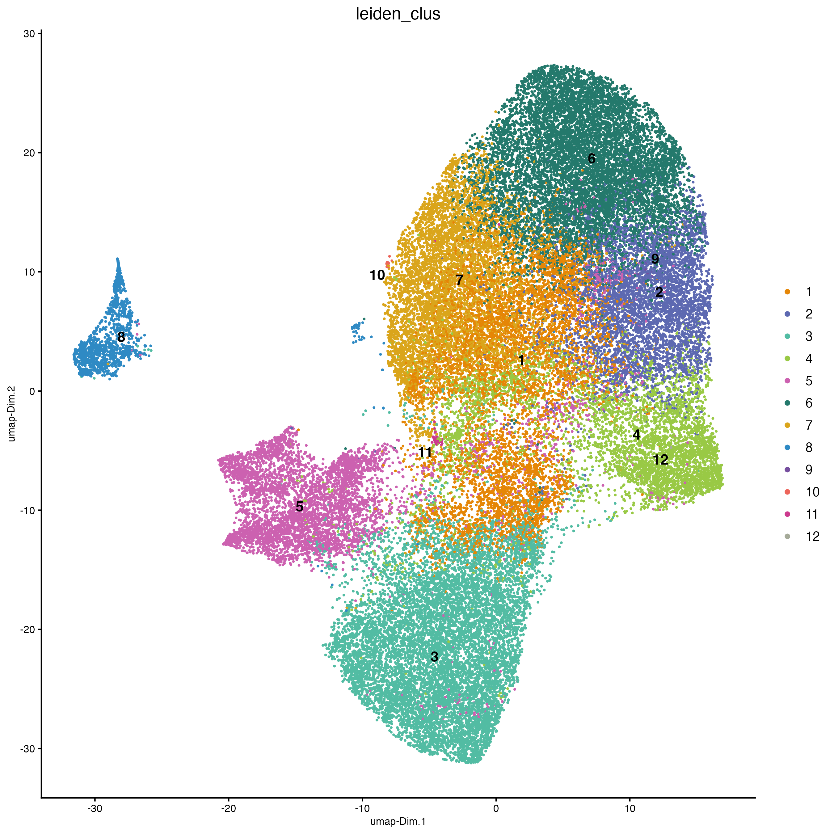
12 Cluster
12.1 Visualize clustering
cosmx <- createNearestNetwork(cosmx,
    dimensions_to_use = 1:10,
    k = 10
)

cosmx <- doLeidenCluster(cosmx,
    resolution = 0.2,
    n_iterations = 100
)

clus_colors <- getColors("Vivid", 12)

# visualize UMAP cluster results
plotUMAP(cosmx,
    cell_color = "leiden_clus",
    cell_color_code = clus_colors,
    point_border_stroke = 0,
    point_size = 1
)
plotTSNE(cosmx,
    cell_color = "leiden_clus",
    cell_color_code = clus_colors,
    point_border_stroke = 0,
    point_size = 1
)
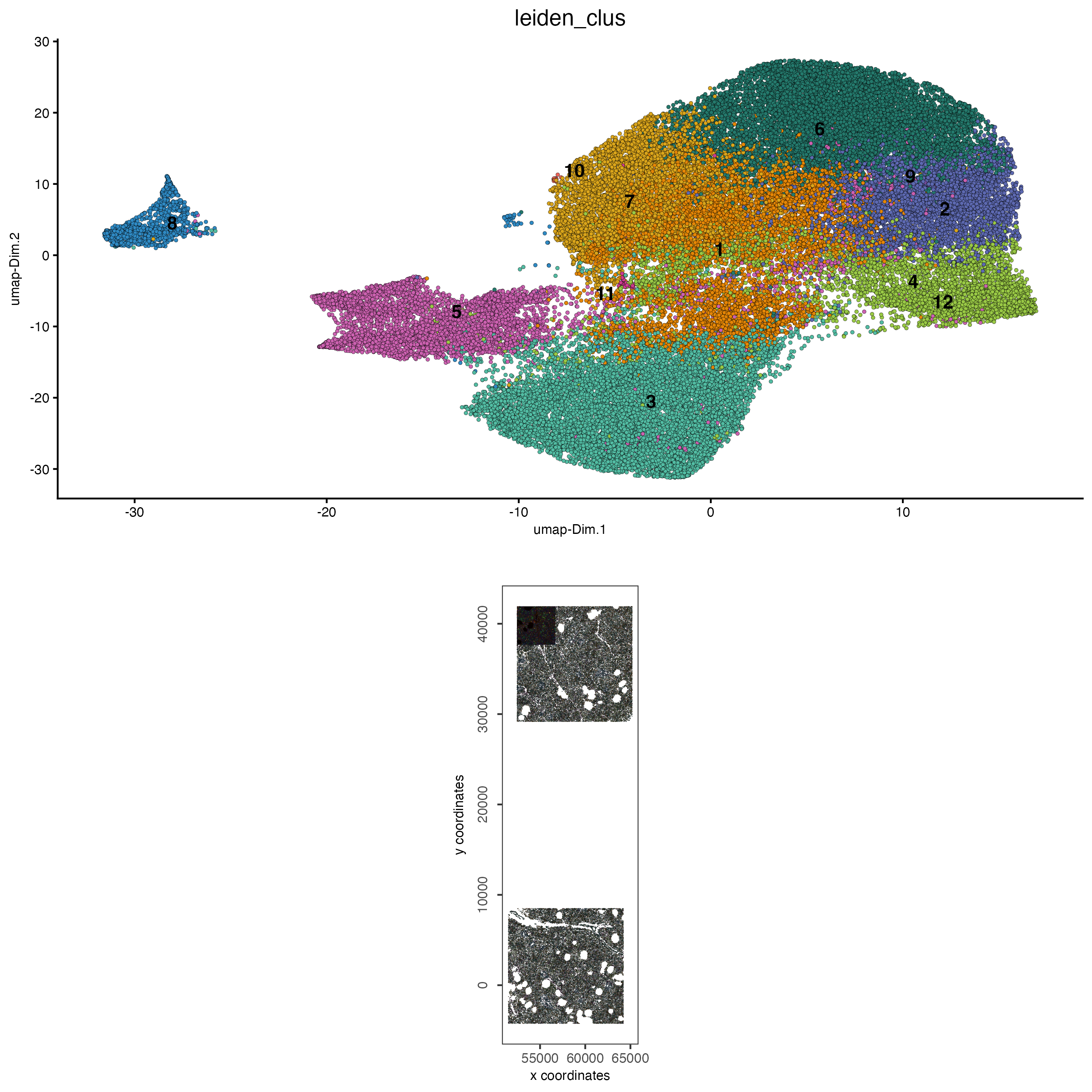
12.2 Visualize clustering on expression and spatial space
# visualize UMAP and spatial results
spatDimPlot2D(cosmx,
    show_image = TRUE,
    cell_color = "leiden_clus",
    cell_color_code = clus_colors,
    spat_point_size = 0.1
)
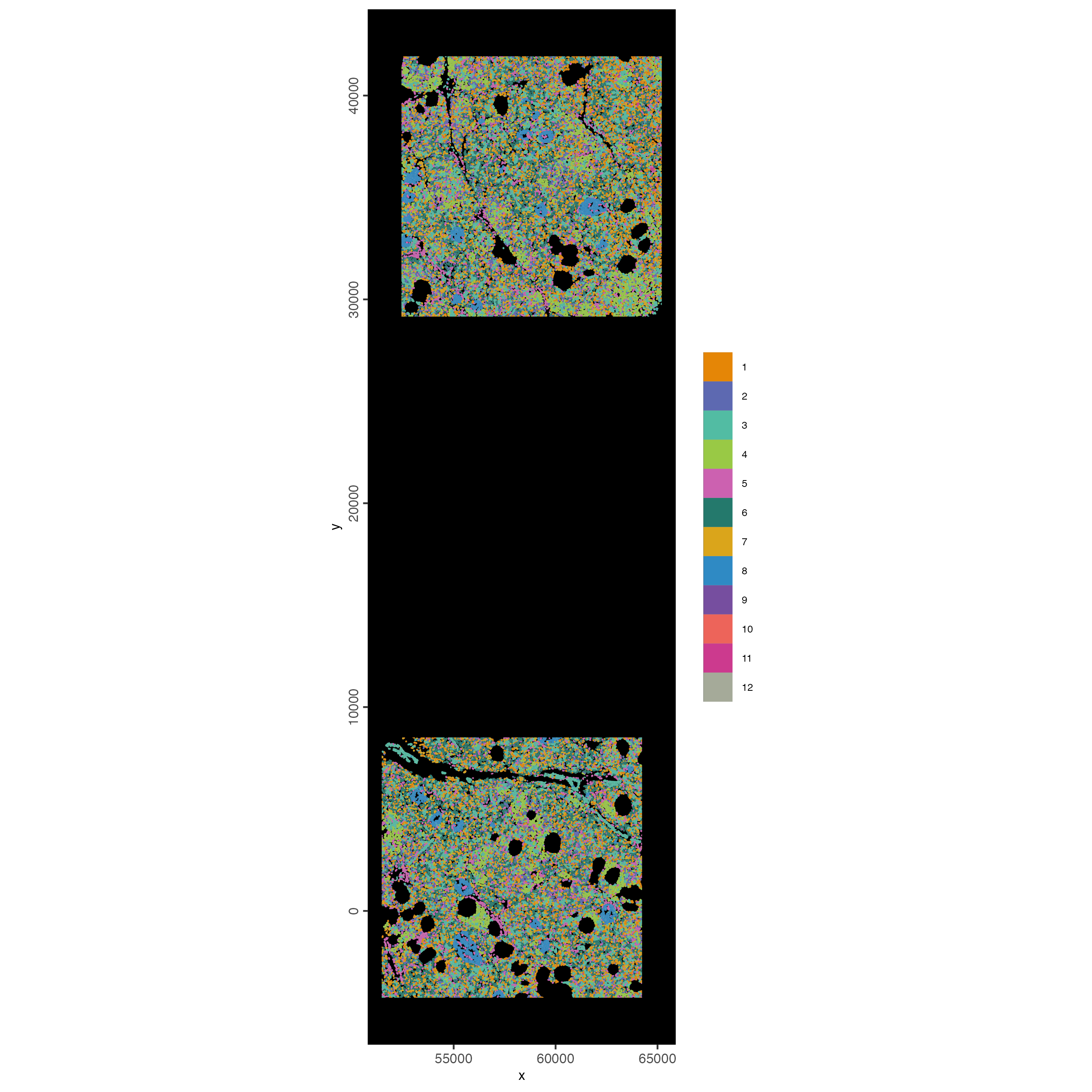
12.3 Map clustering spatially
spatInSituPlotPoints(cosmx,
    show_polygon = TRUE,
    polygon_color = "white",
    polygon_line_size = 0.01,
    polygon_fill = "leiden_clus",
    polygon_fill_as_factor = TRUE,
    polygon_fill_code = clus_colors
)
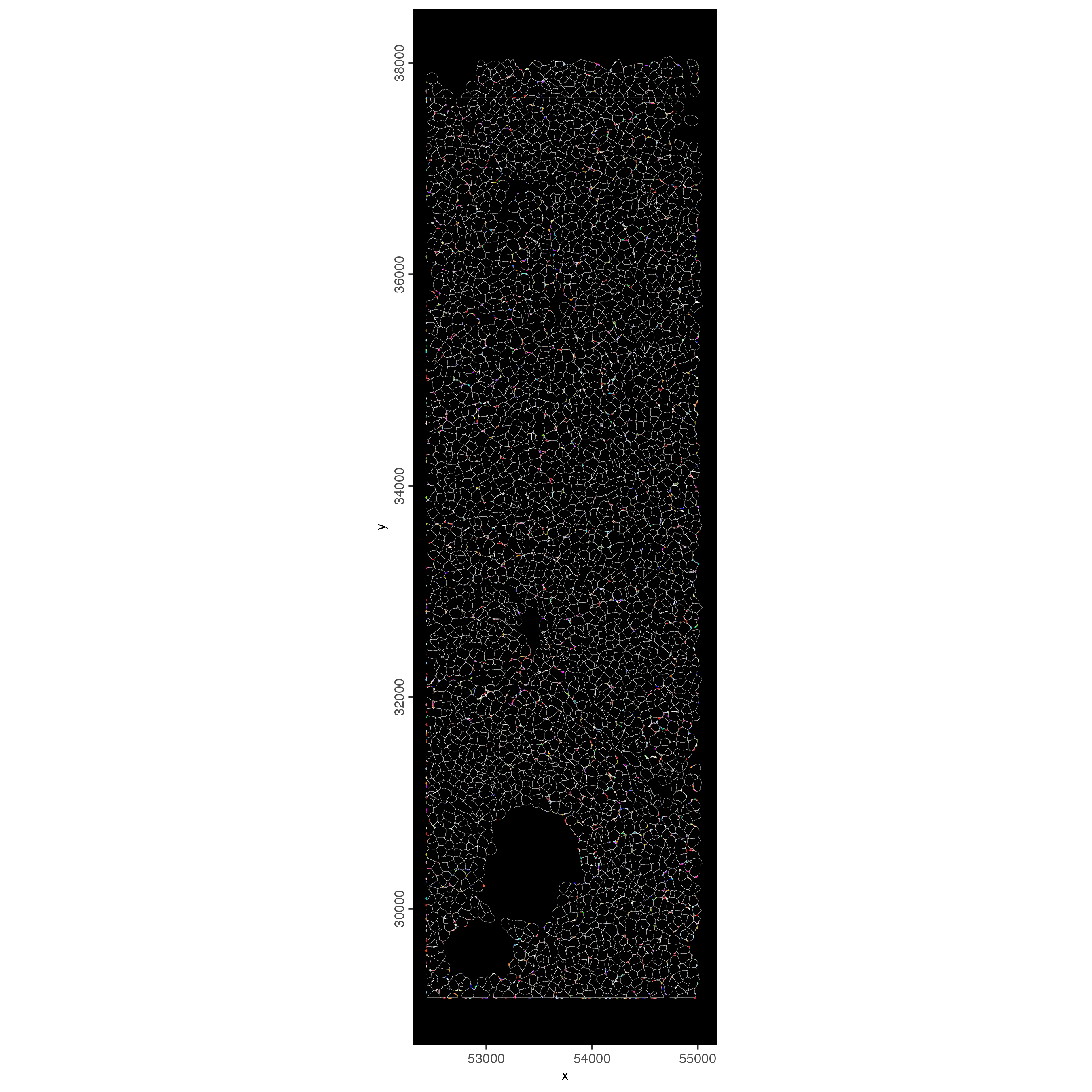
13 Small Subset Visualization
#subset a Giotto object based on spatial locations
smallfov <- subsetGiottoLocs(cosmx,
    x_max = 55000,
    x_min = 45000,
    y_max = 38000,
    y_min = 28000
)

#extract all genes observed in new object
smallfeats <- fDataDT(smallfov)[, feat_ID]

#plot some genes
spatInSituPlotPoints(smallfov,
    feats = list(sample(smallfeats, 400)),
    point_size = 0.5,
    polygon_line_size = 0.05,
    show_polygon = TRUE,
    use_overlap = TRUE,
    polygon_color = "white",
    show_image = FALSE,
    show_legend = FALSE
)
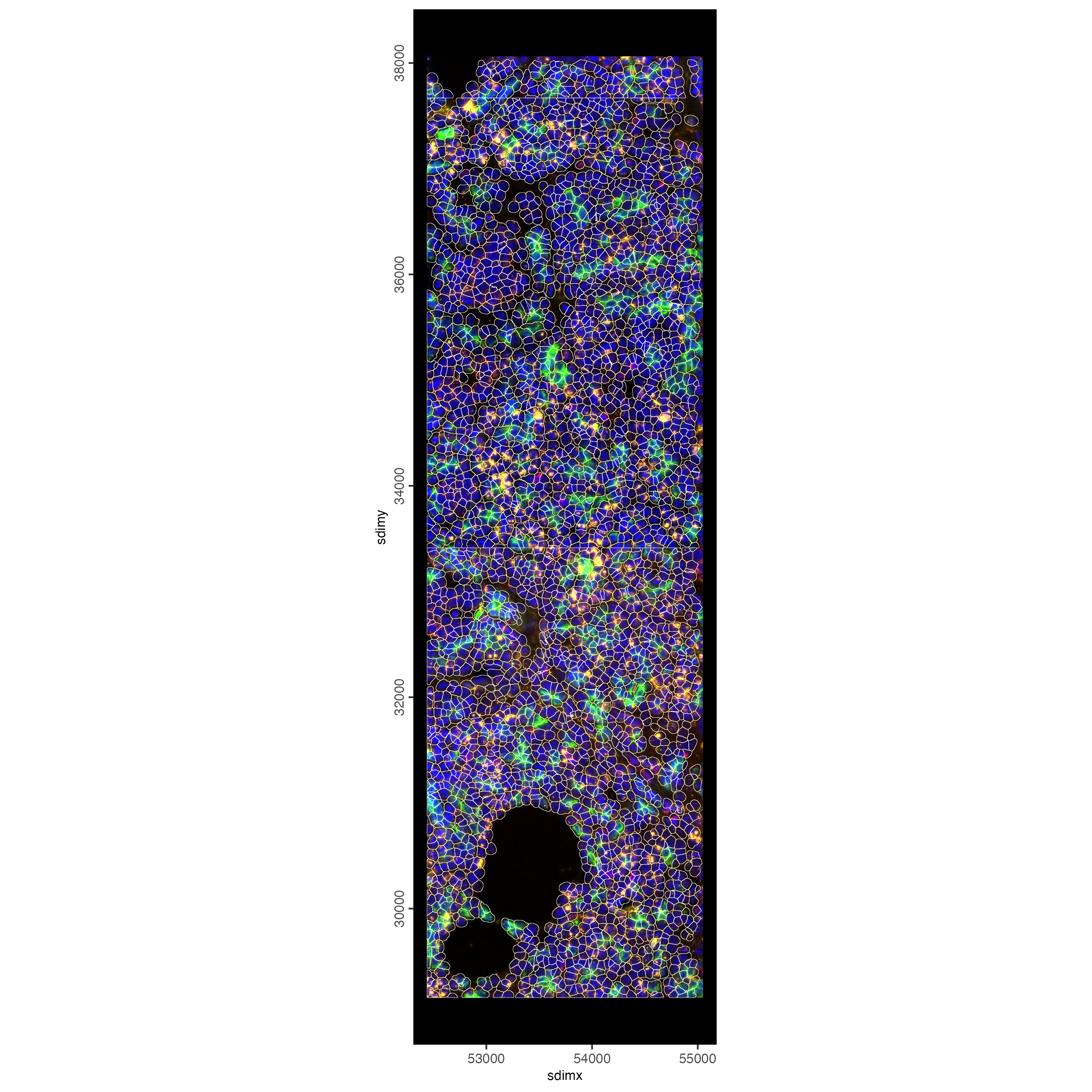
# plot only the polygon outlines
spatInSituPlotPoints(smallfov,
    polygon_line_size = 0.1,
    polygon_alpha = 0,
    polygon_color = "white",
    show_polygon = TRUE,
    show_image = TRUE,
    image_name = c("composite_fov051", "composite_fov052",
                   "composite_fov053"),
    show_legend = FALSE
)
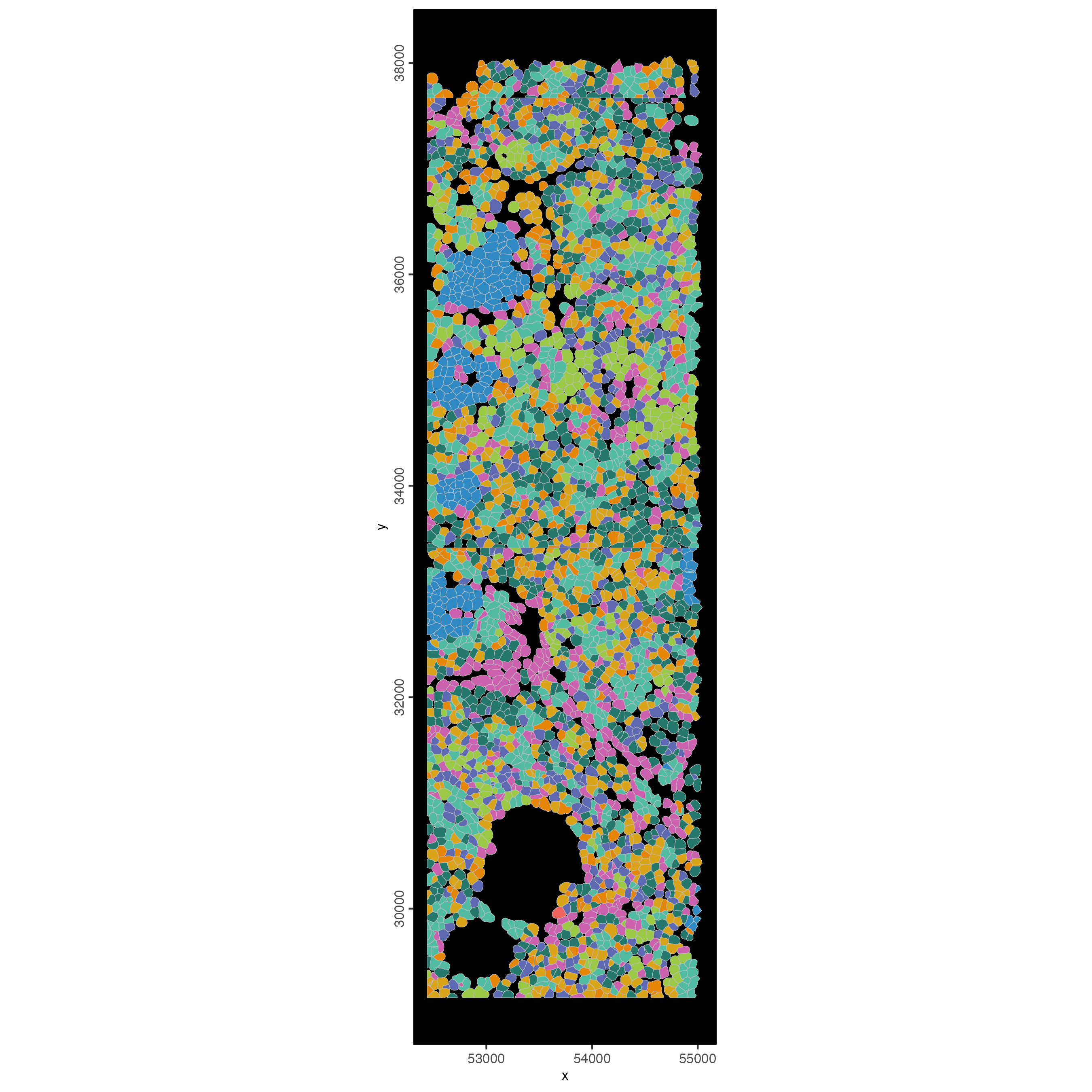
# plot polygons colorlabeled with leiden clusters
spatInSituPlotPoints(smallfov,
    polygon_line_size = 0.1,
    show_polygon = TRUE,
    polygon_fill = "leiden_clus",
    polygon_fill_as_factor = TRUE,
    polygon_fill_code = clus_colors,
    show_image = FALSE,
    show_legend = FALSE
)
14 Session Info
R version 4.5.1 (2025-06-13)
Platform: x86_64-apple-darwin20
Running under: macOS Tahoe 26.2

Matrix products: default
BLAS:   /System/Library/Frameworks/Accelerate.framework/Versions/A/Frameworks/vecLib.framework/Versions/A/libBLAS.dylib
LAPACK: /Library/Frameworks/R.framework/Versions/4.5-x86_64/Resources/lib/libRlapack.dylib;  LAPACK version 3.12.1

locale:
[1] en_US.UTF-8/en_US.UTF-8/en_US.UTF-8/C/en_US.UTF-8/en_US.UTF-8

time zone: America/New_York
tzcode source: internal

attached base packages:
[1] stats     graphics  grDevices utils     datasets  methods   base

other attached packages:
[1] Giotto_4.2.3      GiottoClass_0.5.0

loaded via a namespace (and not attached):
  [1] colorRamp2_0.1.0            gridExtra_2.3
  [3] rlang_1.1.6                 magrittr_2.0.4
  [5] RcppAnnoy_0.0.22            GiottoUtils_0.2.5
  [7] matrixStats_1.5.0           compiler_4.5.1
  [9] systemfonts_1.3.1           png_0.1-8
 [11] vctrs_0.6.5                 pkgconfig_2.0.3
 [13] SpatialExperiment_1.20.0    fastmap_1.2.0
 [15] backports_1.5.0             magick_2.9.0
 [17] XVector_0.50.0              labeling_0.4.3
 [19] ggraph_2.2.2                rmarkdown_2.30
 [21] ragg_1.5.0                  purrr_1.2.0
 [23] xfun_0.55                   bluster_1.20.0
 [25] beachmat_2.26.0             cachem_1.1.0
 [27] jsonlite_2.0.0              DelayedArray_0.36.0
 [29] BiocParallel_1.44.0         tweenr_2.0.3
 [31] terra_1.8-86                irlba_2.3.5.1
 [33] parallel_4.5.1              cluster_2.1.8.1
 [35] R6_2.6.1                    RColorBrewer_1.1-3
 [37] reticulate_1.44.1           parallelly_1.46.0
 [39] rcartocolor_2.1.2           GenomicRanges_1.62.1
 [41] scattermore_1.2             Rcpp_1.1.0
 [43] Seqinfo_1.0.0               SummarizedExperiment_1.40.0
 [45] knitr_1.50                  future.apply_1.20.1
 [47] R.utils_2.13.0              IRanges_2.44.0
 [49] Matrix_1.7-4                igraph_2.2.1
 [51] tidyselect_1.2.1            rstudioapi_0.17.1
 [53] abind_1.4-8                 yaml_2.3.12
 [55] viridis_0.6.5               codetools_0.2-20
 [57] listenv_0.10.0              lattice_0.22-7
 [59] tibble_3.3.0                Biobase_2.70.0
 [61] withr_3.0.2                 S7_0.2.1
 [63] Rtsne_0.17                  evaluate_1.0.5
 [65] future_1.68.0               polyclip_1.10-7
 [67] pillar_1.11.1               MatrixGenerics_1.22.0
 [69] checkmate_2.3.3             stats4_4.5.1
 [71] dbscan_1.2.4                plotly_4.11.0
 [73] generics_0.1.4              S4Vectors_0.48.0
 [75] ggplot2_4.0.1               scales_1.4.0
 [77] gtools_3.9.5                globals_0.18.0
 [79] glue_1.8.0                  lazyeval_0.2.2
 [81] tools_4.5.1                 GiottoVisuals_0.2.14
 [83] BiocNeighbors_2.4.0         data.table_1.17.8
 [85] RSpectra_0.16-2             ScaledMatrix_1.18.0
 [87] graphlayouts_1.2.2          tidygraph_1.3.1
 [89] cowplot_1.2.0               grid_4.5.1
 [91] tidyr_1.3.2                 colorspace_2.1-2
 [93] SingleCellExperiment_1.32.0 BiocSingular_1.26.1
 [95] ggforce_0.5.0               rsvd_1.0.5
 [97] cli_3.6.5                   textshaping_1.0.4
 [99] S4Arrays_1.10.1             viridisLite_0.4.2
[101] dplyr_1.1.4                 uwot_0.2.4
[103] gtable_0.3.6                R.methodsS3_1.8.2
[105] digest_0.6.39               progressr_0.18.0
[107] BiocGenerics_0.56.0         SparseArray_1.10.6
[109] ggrepel_0.9.6               rjson_0.2.23
[111] htmlwidgets_1.6.4           farver_2.1.2
[113] R.oo_1.27.1                 memoise_2.0.1
[115] htmltools_0.5.9             lifecycle_1.0.4
[117] httr_1.4.7                  MASS_7.3-65